Aperta walkthrough: walking accessibility in Central Paris¶
This notebook is a guided tour of every aperta primitive on a real-world example: walking accessibility to supermarkets across Central Paris (arrondissements 1–7 — the historic core of the city: Louvre, Bourse, Marais, Latin Quarter, Saint-Germain, Invalides, ~14 km²). It takes ~1 minute on a laptop. All data is pulled from public sources (OpenStreetMap via OSMnx; Uber’s H3 grid system); no authentication or external downloads beyond pip install are needed.
For a shorter introduction (~40 lines, ~10 s), see `minimal/accessibility.ipynb <../minimal/accessibility.ipynb>`__. For calibration + traffic-flow tuning on a large real network, see `calibration/ <../calibration/>`__ (requires ground-truth data).
The notebook follows aperta’s six-phase workflow:
Load and prepare data — OSM walking network, building footprints (as a synthetic population proxy), and supermarket POIs.
Map data to units — Uber H3 hex cells (resolution 10, ~66 m edge) and parent zones (resolution 8, ~460 m edge). H3’s native parent-child relationship makes the cell→zone mapping deterministic and zero-cost.
Build sparse OD pairs — Three tiers based on zone-pair distance:
cells_to_cells(close — both endpoints at cell precision),cells_to_zones(medium — cell origin, zone-aggregated dest),zones_to_zones(far — both endpoints at zone precision). The middle tier preserves per-cell origin precision in the regime where cell variation matters relative to trip cost.(skipped here) Estimate traffic flows — not relevant for walking.
Estimate travel costs — Dijkstra shortest paths over the walking graph (scipy
csgraph.dijkstra, FP32 by default).Calculate accessibilities — Cumulative-opportunity, gravity, and nearest-k metrics.
The same code structure works for any city anywhere in the world — only the area-of-interest string needs to change.
[1]:
# `%matplotlib inline` makes figures show up inline below each cell when
# running in a Jupyter kernel; `autoreload` re-imports modules when their
# source changes on disk, so library edits don't require a kernel restart.
# All three are IPython magics — no-ops when running this file as plain Python.
%matplotlib inline
%load_ext autoreload
%autoreload 2
[2]:
import warnings

import geopandas as gpd
import h3
import matplotlib.pyplot as plt
import numpy as np
import osmnx as ox
import pandas as pd
from shapely.geometry import Polygon

import aperta.accessibility as accessibility
import aperta.geo_mapping as geo_mapping
import aperta.geo_processing as geo_processing
import aperta.network_processing as network_processing
import aperta.network_snap as network_snap
import aperta.od_pairs as od_pairs
import aperta.overhead as overhead
import aperta.routing as routing
import aperta.routing_prep as routing_prep
import aperta.utility as utility
import aperta.visualization as viz

warnings.filterwarnings('ignore', category=FutureWarning)
1. Area of interest¶
[3]:
# OSMnx accepts a list of place names — the area-of-interest becomes the
# union of all listed polygons. For Central Paris we explicitly enumerate
# the seven historic arrondissements (the alternative `'Paris, France'`
# returns all 20, ~10× the network).
PLACE = [f'Paris {n} Arrondissement, France'
         for n in ('1er', '2e', '3e', '4e', '5e', '6e', '7e')]
LOCATION_LABEL = 'Central Paris (arrondissements 1–7)'
H3_RES_CELLS = 10  # ~66 m hex edge — building-block scale
H3_RES_ZONES = 8   # ~460 m hex edge — small-neighbourhood scale

# OSMnx returns the place polygon in WGS84 (EPSG:4326). When `PLACE` is a
# list, `geocode_to_gdf` returns one row per place — dissolve to a single
# union polygon so downstream code can treat the AOI uniformly.
boundary = ox.geocode_to_gdf(PLACE).dissolve()
boundary_proj_crs = boundary.estimate_utm_crs()  # local metric CRS

print(f"Place:          {LOCATION_LABEL}")
print(f"Projected CRS:  {boundary_proj_crs}")
Place:          Central Paris (arrondissements 1–7)
Projected CRS:  EPSG:32631
2. Build H3 hex grids: cells and zones¶
Uber’s H3 is a hierarchical hex-grid system. Each H3 cell at resolution N has a deterministic parent at resolution N–1, N–2, … — no spatial join needed for the cell→zone mapping.
[4]:
boundary_geom = boundary.geometry.iloc[0]
cells = geo_processing.build_h3_grid(
    boundary_geom, H3_RES_CELLS,
    polygon_crs='EPSG:4326',
    target_crs=boundary_proj_crs,
)
# Each cell's parent at the zone resolution gives its zone assignment.
cells['zone_id'] = [h3.cell_to_parent(c, H3_RES_ZONES) for c in cells.index]

# Zones materialised from the unique zone parents.
zone_ids = sorted(cells['zone_id'].unique())
zones = gpd.GeoDataFrame(
    {'geometry': [Polygon([(lng, lat) for lat, lng in h3.cell_to_boundary(z)])
                  for z in zone_ids]},
    index=pd.Index(zone_ids, name='zone_id'),
    crs='EPSG:4326',
).to_crs(boundary_proj_crs)

print(f"{len(cells):,} cells in {len(zones):,} zones")
1,074 cells in 31 zones
3. Fetch OSM data¶
Three pulls: the walking network (for routing), building footprints (used as a synthetic population proxy), and supermarket POIs (destinations).
A note on the network filter. The intuitive choice is network_type='walk', which excludes motorways and trunk roads. In practice this often produces small disconnected pedestrian islands at city boundaries: pedestrian-only paths (highway=path, foot=designated) that connect to the main grid only via a trunk-tagged road get orphaned when that road is filtered out, and OSMnx’s default retain_all=False then drops them as non-largest components. The cleaner choice for accessibility
analyses in well-mapped urban areas is network_type='all' — it keeps trunk roads (so the pedestrian paths stay connected) at the cost of letting the router walk along trunk roads in the (rare) cases where that’s the shortest path. prepare_network (below) handles the trunk-road problem by tagging motorway / trunk edges as cost-excluded for the walk mode so the walk weight function masks them at ∞.
A second consideration is directedness. graph_from_place returns a MultiDiGraph with directed edges that respect one-way tags — fine for cars, but wrong for walking (pedestrians ignore one-ways). And on a consolidated network, OSMnx’s directed edges can occasionally leave a node trapped in a short one-way segment with no escape — silently producing zero-accessibility outliers in the affected cells. prepare_network(graph, 'walk') handles both: it applies to_undirected() and
precomputes the largest connected component as the snap-eligible node set.
[5]:
# Network. `graph_from_place` returns a MultiDiGraph clipped to the place
# polygon; `prepare_network` then applies the walk-specific defaults:
# undirected routing graph + snap-eligible-nodes + cost-excluded-edges
# (motorway / trunk).
graph = ox.graph_from_place(PLACE, network_type='all', simplify=True)
graph = ox.project_graph(graph, to_crs=boundary_proj_crs)
prepared = routing_prep.prepare_network(graph, 'walk')
graph = prepared.graph
print(f"Network: {graph.number_of_nodes():,} nodes, {graph.number_of_edges():,} edges")
Network: 20,534 nodes, 33,214 edges
[6]:
# Building footprints — synthetic population proxy.
# In a real analysis, replace this with gridded population (GHSL, WorldPop).
# Project to a metric CRS before computing centroids — centroid in geographic
# CRS is geometrically meaningless.
_b = ox.features_from_place(PLACE, tags={'building': True})
_b = _b[_b.geometry.type.isin(['Polygon', 'MultiPolygon'])][['geometry']].to_crs(boundary_proj_crs)
buildings = gpd.GeoDataFrame(
    geometry=_b.geometry.centroid.values,
    index=pd.Index(range(len(_b)), name='building_id'),
    crs=boundary_proj_crs,
)
print(f"{len(buildings):,} building footprints (centroids used as population pseudo-points)")
18,871 building footprints (centroids used as population pseudo-points)
[7]:
# Supermarket POIs — destinations of interest for the accessibility analysis.
_s = ox.features_from_place(PLACE, tags={'shop': 'supermarket'}).to_crs(boundary_proj_crs)
supermarkets = gpd.GeoDataFrame(
    geometry=_s.geometry.centroid.values,
    index=pd.Index(range(len(_s)), name='supermarket_id'),
    crs=boundary_proj_crs,
)
print(f"{len(supermarkets):,} supermarkets")
66 supermarkets
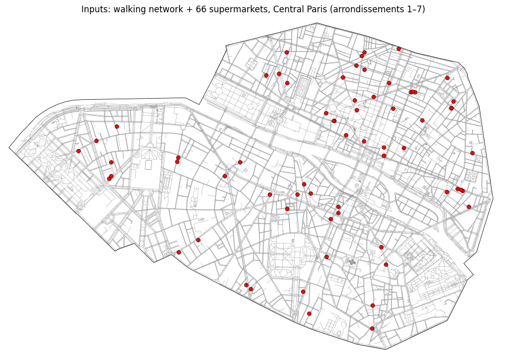
A quick look at the inputs: the walking network (grey edges) and the supermarket destinations (red), inside the AOI boundary.
[8]:
fig, ax = plt.subplots(figsize=(10, 10))
ox.plot_graph(
    graph, ax=ax, node_size=0,
    edge_color='gray', edge_linewidth=0.3,
    bgcolor='white', show=False, close=False,
)
boundary.to_crs(boundary_proj_crs).boundary.plot(
    ax=ax, color='black', linewidth=0.6,
)
supermarkets.plot(
    ax=ax, color='red', markersize=30,
    edgecolor='black', linewidth=0.5, zorder=10,
)
ax.set_title(f'Inputs: walking network + {len(supermarkets)} supermarkets, {LOCATION_LABEL}')
ax.set_axis_off()
plt.tight_layout()
plt.show()
4. Map data to canonical units¶
Three mappings: cells (and zones) get nearest network nodes; buildings and supermarkets get assigned to the cell whose polygon contains them.
[9]:
# Walking speed in m/s (OSMnx default; used both for edge routing and for the
# cell→node walking-overhead estimate below).
WALK_SPEED_MS = 1.4

# Snap each cell's centroid to its nearest network node. `snap_to_network_nodes`
# returns both the node ID and the Euclidean distance from the cell centroid to
# that node — exactly what we need for the per-cell trip-overhead estimate.
cell_centroids_gdf = gpd.GeoDataFrame(
    geometry=cells.geometry.centroid, index=cells.index, crs=cells.crs,
)
cells['node_id'], dist_to_node = network_snap.snap_to_network_nodes(
    cell_centroids_gdf, graph,
    eligible_node_ids=prepared.snap_eligible_nodes,
)
# Walking overhead is the centroid→node distance divided by walking speed.
# Aperta's accessibility cell-mode adds this to every destination cost so that
# two cells sharing the same network node still report different accessibilities.
cells['walk_overhead_s'] = dist_to_node / WALK_SPEED_MS
Zone snapping via tiered transport centroid. Naively snapping each zone’s geometric centroid to the nearest node often lands on something arbitrary — a service road behind a building, a cul-de-sac, or (with network_type='all') even a motorway on-ramp. For zones at ~460 m H3 hex resolution covering heterogeneous urban geometry, this matters: the zone-representative node anchors all zone-tier OD-routing AND the routing-based destination-overhead calculations.
The cleaner approach: classify nodes by the highest tier of road that touches them, exclude the top tier (motorways / trunk roads) and the bottom tier (pedestrian-only paths), then snap each zone to the eligible node nearest to the median coordinates of the zone’s eligible interior nodes — the zone’s transport-weighted centroid. This is what transport_centroid (followed by snap_to_network_nodes) does.
[10]:
# Map OSM highway tags to an ordinal road class (1 = pedestrian-only / off-road
# trails, 5 = primary / trunk). Used both for the tier-aware zone snap below
# and the path-first per-edge feature aggregation in §10.
HIGHWAY_CLASS_MAP = {
    'footway': 1, 'pedestrian': 1, 'path': 1, 'steps': 1, 'track': 1,
    'living_street': 2, 'residential': 2,
    'service': 3, 'unclassified': 3, 'tertiary': 3, 'tertiary_link': 3,
    'secondary': 4, 'secondary_link': 4,
    'primary': 5, 'primary_link': 5, 'trunk': 5, 'trunk_link': 5,
    'motorway': 5, 'motorway_link': 5,
}


def edge_road_class(u, v, data) -> float:
    """Per-edge road class. OSMnx stores `highway` as a string or list (for
    edges tagged with multiple types); pick the first and look it up,
    defaulting to 3 (mid-range) for tags we don't know."""
    h = data.get('highway')
    if isinstance(h, list):
        h = h[0] if h else None
    return float(HIGHWAY_CLASS_MAP.get(h, 3))


# Per-node tier = max road class among the node's connected edges.
node_road_class = network_processing.aggregate_edges_to_nodes(
    graph, edge_attribute=edge_road_class, aggregator='max',
)
# Eligible zone-snap targets: nodes whose highest-class touching road is
# residential through secondary (tiers 2–4). Excludes pure-pedestrian-path-only
# nodes (tier 1) — too minor to anchor a zone — and motorway / trunk nodes
# (tier 5) — pedestrians don't realistically arrive at those.
eligible_zone_nodes = node_road_class[
    (node_road_class >= 2) & (node_road_class <= 4)
].index
print(f"{len(eligible_zone_nodes):,} / {graph.number_of_nodes():,} graph nodes "
      f"are eligible as zone-snap targets (tier 2–4).")

# Snap each zone via the median of its eligible interior nodes (transport
# centroid), falling back to the geometric centroid for any zone with no
# eligible node inside.
zone_centroids = network_snap.transport_centroid(
    zones, graph, eligible_node_ids=eligible_zone_nodes,
)
zones['node_id'], _ = network_snap.snap_to_network_nodes(
    zone_centroids, graph, eligible_node_ids=eligible_zone_nodes,
)
7,724 / 20,534 graph nodes are eligible as zone-snap targets (tier 2–4).
[11]:
# Assign each building to the cell whose polygon contains its centroid.
# `allow_nearest=True` catches the rare case of a centroid landing just
# outside the H3 hex coverage; the distance return is unused here.
buildings['cell_id'], _ = geo_mapping.map_points_to_polygons(
    buildings, cells, allow_nearest=True,
)
pop_by_cell = buildings.groupby('cell_id').size()
cells['population'] = pop_by_cell.reindex(cells.index, fill_value=0).astype(float)
[12]:
# Same for supermarkets.
supermarkets['cell_id'], _ = geo_mapping.map_points_to_polygons(
    supermarkets, cells, allow_nearest=True,
)
sm_by_cell = supermarkets.groupby('cell_id').size()
cells['supermarkets'] = sm_by_cell.reindex(cells.index, fill_value=0).astype(float)
[13]:
# Aggregate destination weights up to the zone level so the zone tier carries
# the right per-zone totals (one row per zone, summing cells below it).
zones['population'] = cells.groupby('zone_id')['population'].sum().reindex(
    zones.index, fill_value=0).astype(float)
zones['supermarkets'] = cells.groupby('zone_id')['supermarkets'].sum().reindex(
    zones.index, fill_value=0).astype(float)

print(f"Total pseudo-population: {cells['population'].sum():,.0f} buildings")
print(f"Cells with at least one supermarket: {(cells['supermarkets'] > 0).sum()}")
Total pseudo-population: 18,871 buildings
Cells with at least one supermarket: 59
5. Build tiered origin-destination pairs¶
Three radii classify every zone-pair into one of three tiers:
cells_to_cells(d(Z, Z') < r_cells): cell origin and cell dest — highest precision, kept small to bound storage.cells_to_zones(r_cells ≤ d < r_medium): cell origin, zone- aggregated dest — preserves per-cell origin precision in the regime where the per-cell dest precision starts being washed out by the trip cost.zones_to_zones(r_medium ≤ d < r_zones): zone-aggregated both sides — cheapest tier, used for far destinations where neither endpoint’s individual cell identity matters much.
r_medium defaults to min(r_cells * 10, r_zones) if not given — we pass it explicitly here so all three tiers are visible.
[14]:
R_CELLS  = 1_500.0   # 1.5 km — cells_to_cells (within ~20 min walking)
R_MEDIUM = 3_000.0   # 3 km   — cells_to_zones middle tier
R_ZONES  = 8_000.0   # 8 km   — zones_to_zones outer cutoff

pairs = od_pairs.get_pairs(
    cells, r_cells=R_CELLS, node_column='node_id',
    zones=zones, r_zones=R_ZONES, r_medium=R_MEDIUM,
)
print(pairs)
TieredODNodePairs(cells_to_cells: 1,074 orig → 325,128 dest; cells_to_zones: 1,074 orig → 15,652 dest; zones_to_zones: 31 orig → 328 dest)
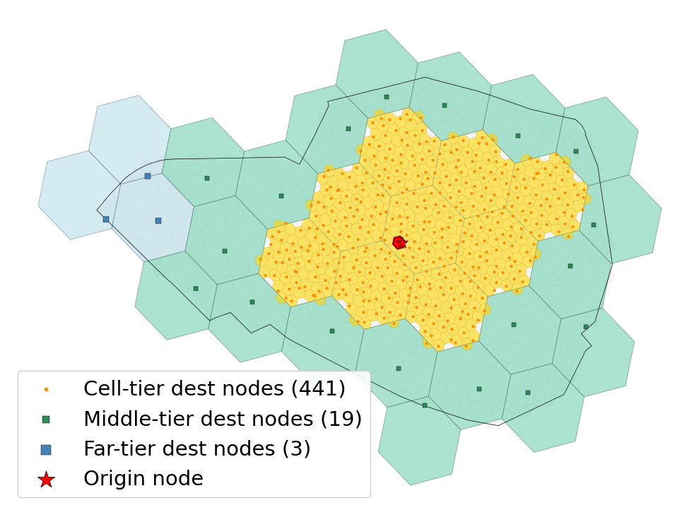
Visualising the tiered structure from one origin. plot_tiered_destinations draws each tier’s destinations in a distinct colour:
Red — origin cell
Gold —
cells_to_cellsdestinations (cell precision)Teal —
cells_to_zonesdestinations (zone-aggregated, mid-distance)Blue —
zones_to_zonesdestinations (zone-aggregated, far)
The three layers fan out concentrically: the per-cell tier is the small high-resolution core, the middle tier is the surrounding annulus of zone-aggregated dests, the far tier is the outer ring (often overlapping the middle tier in the visualisation since the same destination zone may show up at different tiers from different origins). High resolution where it matters, coarser resolution where it doesn’t.
[15]:
# Pick an origin cell near the centre of the AOI for the illustration.
_center = boundary.to_crs(boundary_proj_crs).geometry.iloc[0].centroid
demo_cell_id = cells.geometry.centroid.distance(_center).idxmin()
[16]:
ax = viz.plot_tiered_destinations(
    cells, zones, pairs,
    origin_cell_id=demo_cell_id,
    graph=graph,
    boundary=boundary.to_crs(boundary_proj_crs),
)
_legend = ax.get_legend()
if _legend is not None:
    _handles, _labels = ax.get_legend_handles_labels()
    _legend.remove()
    ax.legend(_handles, _labels,
              loc='lower left', fontsize=21, markerscale=1.5, framealpha=0.9)
plt.tight_layout()
ax.figure.savefig('results/tiered_destinations.pdf', bbox_inches='tight')
plt.show()
6. Compute travel times (Dijkstra over the walking graph)¶
tiered_path_costs routes every OD pair in pairs via scipy.sparse.csgraph.dijkstra (one single-source call per origin) and returns a TieredODNodePairs of cost arrays — same shape as pairs, position-aligned with the per-origin dest arrays.
cutoff=T (optional) caps each per-origin search at T weight-units (seconds here, since edge weight is travel time). Worth using when the graph is much larger than the longest realistic trip: scipy’s limit= parameter truncates the Dijkstra frontier once it exceeds T, which can be a big speed-up on country-scale networks. At Central Paris scale (graph diameter ≈ 30 min walking) the cutoff barely matters, but we set it for illustration.
Output dtype is np.float32 by default (halves storage versus FP64 with no meaningful precision loss for travel costs in seconds). Pass dtype=np.float64 if downstream arithmetic needs the extra range.
[17]:
# Convert each edge's length (m) into a walking time (s). `mask_excluded_edges`
# wraps the per-edge callable so motorway / trunk edges (flagged by
# `prepare_network`) get cost = ∞ — making them effectively unwalkable for the
# routing engine.
walk_weight = routing.mask_excluded_edges(
    lambda d: d['length'] / WALK_SPEED_MS, prepared.cost_excluded_flag,
)
routing.apply_edge_weights(graph, walk_weight, 'walk_time_s')

times = routing.tiered_path_costs(graph, pairs, weight='walk_time_s',
    cutoff=45 * 60,  # 45 min upper bound; r_zones * (1/walk_speed) gives ≈30 min
)
print(times)
TieredODNodePairs(cells_to_cells: 1,074 orig → 325,128 dest; cells_to_zones: 1,074 orig → 15,652 dest; zones_to_zones: 31 orig → 328 dest)
7. Lift to geo-keyed form, bake per-cell overhead, build weights¶
Routing produces a node-keyed TieredODNodePairs — keys are network node IDs. To get per-cell accessibility output, baked per-cell origin overhead, or cross-modal aggregation across different graphs, lift to TieredODGeoPairs (keys = cell IDs / zone IDs).
Three steps:
reindex_by_geo_unit— fan out node-keyed entries to cell/zone entries.add_geo_overheads— bake per-cell first-mile into the cost ODM. Passingorigin_cell=alone is enough: the helper auto-derives the zone-tier overhead as the group-mean of the per-cell values, using thecell_to_zonemap. Cells and zones share the same first-mile intent — per-cell atcells_to_cells/cells_to_zonesand per-zone-mean atzones_to_zones(the far tier is keyed by zone, not cell).lookup_dest_column_geo— build per-cell destination weight ODMs directly.
[18]:
pairs_geo, times_geo = od_pairs.reindex_by_geo_unit(
    pairs, times, cells,
    cell_node_column='node_id',
    zones=zones, zone_node_column='node_id',
    r_cells=R_CELLS, r_medium=R_MEDIUM, r_zones=R_ZONES,
)
times_geo = overhead.add_geo_overheads(
    times_geo, pairs_geo,
    origin_cell=cells['walk_overhead_s'],
    cell_to_zone=cells['zone_id'],
)
sm_weights = od_pairs.lookup_dest_column_geo(
    'supermarkets', pairs_geo, cells, zones=zones,
)
# Cell → zone lookup for tier stitching in the accessibility metrics.
cell_to_zone = cells['zone_id'].to_dict()

print(times_geo)
TieredODGeoPairs(cells_to_cells: 1,074 orig → 325,128 dest; cells_to_zones: 1,074 orig → 15,652 dest; zones_to_zones: 31 orig → 328 dest)
8. Accessibility metrics¶
Three flavours, computed against the geo-keyed cost ODM with overhead baked in. Output is indexed by cell ID — ready to join back to the cells GeoDataFrame for mapping. No per-call cells= / node_column= / cell_overhead_column= kwargs needed — the geo-keyed input does the work.
Cumulative-opportunity: supermarkets reachable per time band¶
[19]:
bins = [
    accessibility.Bin('0_to_5min',   0,           5 * 60),
    accessibility.Bin('5_to_15min',  5 * 60,     15 * 60),
    accessibility.Bin('15_to_30min', 15 * 60,    30 * 60),
]
acc_cum = accessibility.cumulative_opportunities(
    times_geo, {'supermarkets': sm_weights}, cell_to_zone, bins,
)

# Cumulative variant — supermarkets reachable WITHIN X minutes.
acc_within = pd.DataFrame({
    'within_5min':  acc_cum[('0_to_5min', 'supermarkets')],
    'within_15min': (acc_cum[('0_to_5min', 'supermarkets')]
                     + acc_cum[('5_to_15min', 'supermarkets')]),
    'within_30min': (acc_cum[('0_to_5min', 'supermarkets')]
                     + acc_cum[('5_to_15min', 'supermarkets')]
                     + acc_cum[('15_to_30min', 'supermarkets')]),
})
acc_within.head()
[19]:
| within_5min | within_15min | within_30min | |
|---|---|---|---|
| cell | |||
| 8a1fb4644c37fff | 0.0 | 0.0 | 26.0 |
| 8a1fb4644cb7fff | 0.0 | 2.0 | 18.0 |
| 8a1fb4644d07fff | 0.0 | 5.0 | 35.0 |
| 8a1fb4644d17fff | 0.0 | 3.0 | 28.0 |
| 8a1fb4644d1ffff | 0.0 | 1.0 | 23.0 |
Gravity: exponential decay, three β values in one call¶
The cost ODM is floored at 30 s via floor_intrazonal_costs before passing to gravity. Without that floor, the intrazonal self-pair would route at cost 0, sending exp(-β · 0) = 1 to maximum decay weight (giving a cell’s own supermarkets infinite advantage over neighbours).
[20]:
times_geo_floored = routing.floor_intrazonal_costs(times_geo, min_cost=30.0)

decays = [
    accessibility.exp_decay('beta_005', 0.005),  # half-decay ~140 s ≈ 2 min
    accessibility.exp_decay('beta_002', 0.002),  # half-decay ~350 s ≈ 6 min
    accessibility.exp_decay('beta_001', 0.001),  # half-decay ~700 s ≈ 12 min
]
acc_gravity = accessibility.gravity(
    times_geo_floored, {'supermarkets': sm_weights}, cell_to_zone, decays,
)
acc_gravity.head()
[20]:
| decay | beta_005 | beta_002 | beta_001 |
|---|---|---|---|
| property | supermarkets | supermarkets | supermarkets |
| cell | |||
| 8a1fb4644c37fff | 0.062612 | 2.269983 | 10.191812 |
| 8a1fb4644cb7fff | 0.057568 | 1.912636 | 9.177878 |
| 8a1fb4644d07fff | 0.190554 | 3.179389 | 11.795935 |
| 8a1fb4644d17fff | 0.122867 | 3.028626 | 11.736505 |
| 8a1fb4644d1ffff | 0.068637 | 2.424563 | 10.570081 |
Nearest-k: mean walking time to the k nearest supermarkets¶
Default aggregator is 'cost_mean' — the mean cost over the k nearest weight-units (each supermarket counts as one opportunity at its destination’s cost). Lower values = better accessibility, and k = 3 and k = 5 are directly comparable on the same (seconds) scale. Cells with fewer than k reachable supermarkets show NaN.
[21]:
acc_nk = accessibility.nearest_k(
    times_geo, {'supermarkets': sm_weights}, cell_to_zone, ks=[1, 3, 5],
)
acc_nk.head()
[21]:
| k | 1 | 3 | 5 |
|---|---|---|---|
| property | supermarkets | supermarkets | supermarkets |
| cell | |||
| 8a1fb4644c37fff | 903.913147 | 928.268066 | 965.768250 |
| 8a1fb4644cb7fff | 829.353699 | 870.396667 | 980.908020 |
| 8a1fb4644d07fff | 605.854004 | 686.646423 | 704.528442 |
| 8a1fb4644d17fff | 725.996521 | 802.627136 | 867.709778 |
| 8a1fb4644d1ffff | 858.657593 | 930.931580 | 979.907410 |
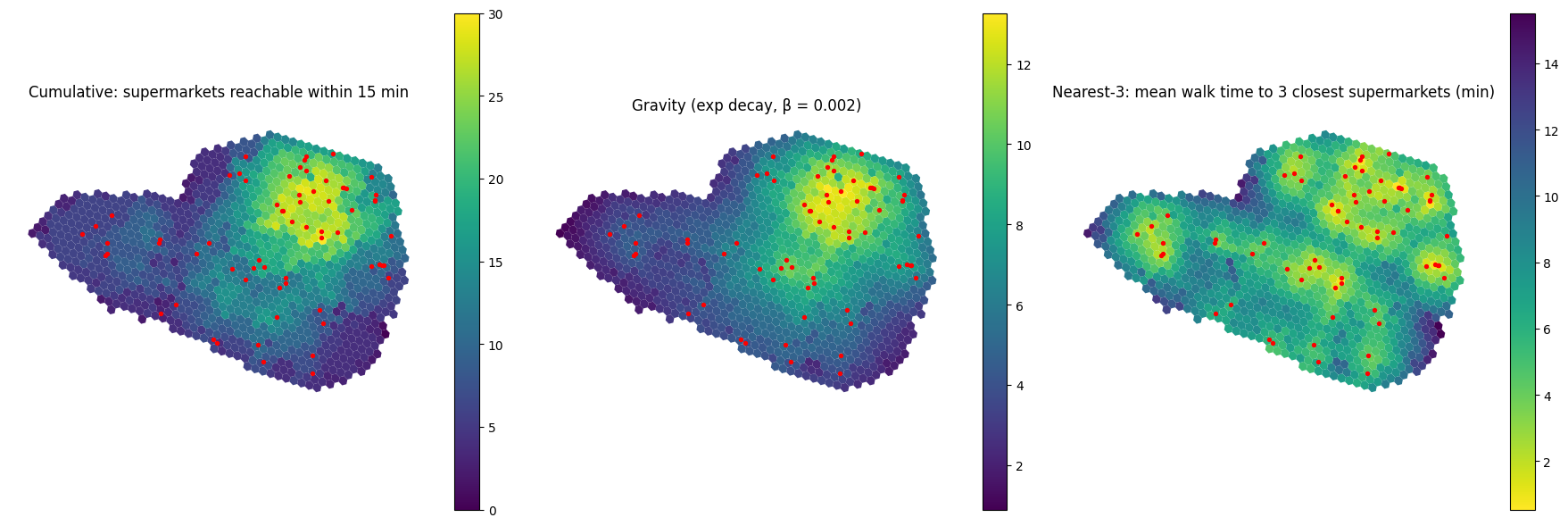
9. Visualise¶
Three choropleths, one per metric family. Cells with their accessibility value as fill colour; supermarket locations overlaid.
[22]:
# Three panels, three metrics. The first two are "bigger = better"; the
# third (nearest-3 cost in minutes) is "smaller = better", so we use a
# reversed colormap to keep the visual convention "bright = good" consistent.
fig, axes = plt.subplots(1, 3, figsize=(18, 6))
sm_overlay = [(supermarkets, {'color': 'red', 'markersize': 8})]
viz.plot_cell_values(
    cells, acc_within['within_15min'], ax=axes[0],
    title='Cumulative: supermarkets reachable within 15 min',
    overlays=sm_overlay,
)
viz.plot_cell_values(
    cells, acc_gravity[('beta_002', 'supermarkets')], ax=axes[1],
    title='Gravity (exp decay, β = 0.002)',
    overlays=sm_overlay,
)
viz.plot_cell_values(
    cells, acc_nk[(3, 'supermarkets')] / 60, ax=axes[2],
    title='Nearest-3: mean walk time to 3 closest supermarkets (min)',
    cmap='viridis_r',
    overlays=sm_overlay,
)
plt.tight_layout()
plt.show()
10. Adding a bike mode (separate network + intersection-aware edge times)¶
Cycling-walking is the canonical “soft modes” pair for accessibility analyses in dense European city centres — cycling-infrastructure expansion in central Paris (Plan Vélo, cyclable arteries, low-traffic neighbourhoods) is one of the most actively-studied urban-planning topics right now. Compared to walking, biking is ~3× faster but has setup overhead (unlock, parking) and pays a time penalty at every intersection traversed.
This section adds the bike mode end-to-end in the time domain — fetch network, intersection-aware edge times, overhead, route, lift to geo-keyed form, bake overhead. A per-edge bike-friendliness score (used as a route-feature in the utility section later) is computed in §11. The walk + bike utilities + cross-modal logsum follow in §13.
Two new ingredients beyond the walking template:
Edge weights richer than baseline length / speed. Each bike-network edge gets a per-traversal time penalty added to its
length / bike_speedbaseline — every intersection crossed costs a few seconds of stop-and-go. The router uses these penalty-augmented weights, so a slightly-longer detour that avoids one extra intersection can win on total time.An overhead the walking mode doesn’t have. Unlocking the bike
walking to it adds ~30–60 s of trip-invariant cost. For very short trips this can flip the fastest-mode choice back to walking — exactly the cross-modal effect demonstrated in §12.
10.1 Fetch and snap the bike network¶
Same prepare_network pattern as for walk, with mode='bike': applies to_undirected() and snaps to the largest connected component.
Jurisdiction caveat: the 'bike' default applies to_undirected(), which assumes bikes can ride against any one-way street. That holds in Paris, Brussels, Amsterdam etc. (general contraflow cycling allowance) but is too permissive for strict jurisdictions (much of the US, parts of Germany). For a production analysis in a strict jurisdiction the cleaner pattern is prepare_network(bike_graph, 'bike', directedness='directed_scc') — keeps the graph directed AND snaps cells to the
largest strongly-connected component instead of the largest CC. Or use OSM tags (oneway:bicycle=no, cycleway:left= opposite_lane, bicycle:backward=yes) to pre-filter edges so the bike-graph is directed-but-jurisdiction-correct.
[23]:
bike_graph = ox.graph_from_place(PLACE, network_type='bike', simplify=True)
bike_graph = ox.project_graph(bike_graph, to_crs=boundary_proj_crs)
bike_prepared = routing_prep.prepare_network(bike_graph, 'bike')
bike_graph = bike_prepared.graph
print(f"Bike network: {bike_graph.number_of_nodes():,} nodes, "
      f"{bike_graph.number_of_edges():,} edges")

# Per-cell snapping (centroid → nearest bike-network node), capturing the
# centroid→node distance for the per-cell first-mile overhead below.
cells['bike_node_id'], bike_dist_to_node = network_snap.snap_to_network_nodes(
    cell_centroids_gdf, bike_graph,
    eligible_node_ids=bike_prepared.snap_eligible_nodes,
)

# Zone snapping via transport centroid (same tier-aware logic as for walk).
bike_node_road_class = network_processing.aggregate_edges_to_nodes(
    bike_graph, edge_attribute=edge_road_class, aggregator='max',
)
bike_eligible_nodes = bike_node_road_class[
    (bike_node_road_class >= 2) & (bike_node_road_class <= 4)
].index
bike_zone_centroids = network_snap.transport_centroid(
    zones, bike_graph, eligible_node_ids=bike_eligible_nodes,
)
zones['bike_node_id'], _ = network_snap.snap_to_network_nodes(
    bike_zone_centroids, bike_graph, eligible_node_ids=bike_eligible_nodes,
)
Bike network: 3,510 nodes, 5,480 edges
10.2 Intersection-aware edge times¶
Each edge’s bike-time is its length / bike_speed baseline plus a flat per-edge penalty — in a simplified OSMnx graph (every degree-2 node collapsed away), each edge spans exactly one intersection-to-intersection segment, so charging the penalty per edge directly counts intersections along the route. Two effects worth predicting:
The router prefers paths with fewer edges, all else equal.
Routes via longer arterial segments (fewer intersections) get cheaper than dense grid-routes with many short turns.
This is a deliberately tiny example of “edge weights richer than pure length / speed”. For systematic calibration against observed travel times see the separate calibration.ipynb notebook.
[24]:
BIKE_SPEED_MS = 20 / 3.6           # 20 km/h, typical urban cycling speed
INTERSECTION_PENALTY_S = 8.0       # stop-and-go time per intersection traversed

bike_weight = routing.mask_excluded_edges(
    lambda d: float(d['length']) / BIKE_SPEED_MS + INTERSECTION_PENALTY_S,
    bike_prepared.cost_excluded_flag,
)
routing.apply_edge_weights(bike_graph, bike_weight, 'bike_time_s')
10.3 Bike overhead (unlock + walk-to-bike)¶
Per-cell origin overhead = walk-to-bike + fixed setup time. No density-dependent term (unlike cars, bikes don’t need to “find parking” at scale in central Paris).
[25]:
BIKE_INIT_SPEED_MS = 1.4       # walk-to-bike speed
BIKE_SETUP_S = 30.0            # unlock + helmet

cells['bike_overhead_s'] = bike_dist_to_node / BIKE_INIT_SPEED_MS + BIKE_SETUP_S
print(f"Bike overhead per cell: mean {cells['bike_overhead_s'].mean():.1f}s, "
      f"5-95 pct [{cells['bike_overhead_s'].quantile(0.05):.1f}, "
      f"{cells['bike_overhead_s'].quantile(0.95):.1f}]")
Bike overhead per cell: mean 61.8s, 5-95 pct [36.2, 104.8]
10.4 Route, lift to geo, bake overhead¶
Same three-step pattern as the walking pipeline (§6, §7): route on the bike graph → reindex to geo-keyed form → bake per-cell origin overhead into the cost ODM. The result bike_times_geo is a TieredODGeoPairs of bike travel times in seconds with overhead included, ready to combine with times_geo in the cross-modal section that follows.
[26]:
bike_pairs = od_pairs.get_pairs(
    cells, r_cells=R_CELLS, node_column='bike_node_id',
    zones=zones, r_zones=R_ZONES, r_medium=R_MEDIUM,
)
# Note: `r_medium` is passed explicitly so the bike ODM has the SAME
# three-tier structure as the walk ODM. `aggregate_across_modes` (below)
# requires consistent tier structure across modes — without an explicit
# `r_medium`, the bike call would auto-infer `r_medium = min(r_cells * 10,
# r_zones) = r_zones`, collapsing the far tier and crashing the cross-modal
# call.
bike_times = routing.tiered_path_costs(bike_graph, bike_pairs, weight='bike_time_s')
bike_pairs_geo, bike_times_geo = od_pairs.reindex_by_geo_unit(
    bike_pairs, bike_times, cells,
    cell_node_column='bike_node_id',
    zones=zones, zone_node_column='bike_node_id',
    r_cells=R_CELLS, r_medium=R_MEDIUM, r_zones=R_ZONES,
)
bike_times_geo = overhead.add_geo_overheads(
    bike_times_geo, bike_pairs_geo,
    origin_cell=cells['bike_overhead_s'],
    cell_to_zone=cells['zone_id'],
)
print(bike_times_geo)
TieredODGeoPairs(cells_to_cells: 1,074 orig → 325,128 dest; cells_to_zones: 1,074 orig → 15,652 dest; zones_to_zones: 31 orig → 328 dest)
11. Path-first: per-edge feature aggregation along realised routes¶
Everything above used aperta’s cost primitive — routing returns one scalar (travel time) per OD pair, and the accessibility metrics aggregate those scalars. But aperta is also path-first: routing.tiered_path_aggregate routes shortest paths and aggregates any per-edge attribute along each realised path, returning per-OD-pair scalars. Memory cost is the same as tiered_path_costs (paths are processed per-origin and discarded after aggregation).
Concrete use case on the bike network we just built: a bike-friendliness score along each shortest cycling route. We tag each edge 1 (busy primary road) to 5 (dedicated cycleway), combining road tier and OSM cycleway-infrastructure tags. Aggregated by mean along the route, this answers “from this cell, how bike-friendly are the typical routes I’d ride?” — a route-quality metric the cost-only metrics in §8/§9 cannot express, because they see only OD time, not route geometry.
Same primitive applies to any per-edge feature: gradient, surface type, perceived safety, pollution exposure, lit-vs-unlit. Whatever you can attach to an edge, you can aggregate along realised routes. The bike score plays a second role in §13: it enters the bike utility as a RouteFeature, so cyclists value bike-friendly routes proportionally in the discrete-choice accessibility metric.
[27]:
def edge_bike_score(u, v, data) -> float:
    """Per-edge bike-friendliness, 1 (worst) to 5 (best for cycling).

    Combines road tier (quieter = better) with OSM bicycle-infrastructure
    tags. Dedicated cycleways score 5 outright; otherwise the base score
    comes from road tier (inverse of `edge_road_class`: pedestrian = 5,
    residential = 4, ..., primary/motorway = 1), with a +1 / +2 bonus
    for cycleway lane / track on the road, capped at 5.
    """
    h = data.get('highway')
    if isinstance(h, list):
        h = h[0] if h else None
    # Dedicated bike infrastructure wins outright.
    if h == 'cycleway' or data.get('bicycle') == 'designated':
        return 5.0
    # Base score = inverse of road tier (1..5 → 5..1).
    base = 6 - int(edge_road_class(u, v, data))
    # Bonus for any cycleway infrastructure tagged on this road.
    cw = (data.get('cycleway')
          or data.get('cycleway:left')
          or data.get('cycleway:right'))
    if isinstance(cw, list):
        cw = cw[0] if cw else None
    if cw in ('track', 'opposite_track'):
        bonus = 2
    elif cw:                  # 'lane', 'shared', 'opposite_lane', etc.
        bonus = 1
    else:
        bonus = 0
    return float(min(5, base + bonus))


# `PathAggregation` matches the `Bin` / `Decay` namedtuple style used
# elsewhere in aperta: a named spec consisting of an attribute extractor
# and an aggregator. `tiered_path_aggregate` returns both the per-pair
# costs and the per-pair aggregated features — same single routing pass.
_costs, path_aggs = routing.tiered_path_aggregate(bike_graph, bike_pairs, weight='bike_time_s',
    edge_aggregations=[
        routing.PathAggregation('bike_score_avg', edge_bike_score, 'mean'),
    ],
)
bike_score_odm = path_aggs['bike_score_avg']
print(bike_score_odm)
TieredODNodePairs(cells_to_cells: 1,001 orig → 285,365 dest; cells_to_zones: 1,001 orig → 14,615 dest; zones_to_zones: 31 orig → 328 dest)
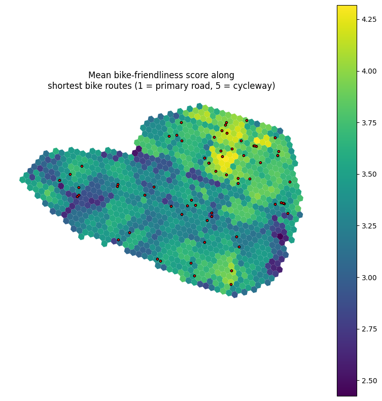
Visualise per origin: unweighted mean across cell-tier destinations. (For a more focused metric, you could weight by supermarkets and only consider routes to supermarket cells; left as an exercise.)
[28]:
per_origin_bike_score = pd.Series(
    {origin: np.nanmean(values)
     for origin, values in bike_score_odm.cells_to_cells.items()},
    name='mean_bike_score_on_rides',
)
per_cell_bike_score = cells['bike_node_id'].map(per_origin_bike_score)

viz.plot_cell_values(
    cells, per_cell_bike_score, cmap='viridis',
    title='Mean bike-friendliness score along\nshortest bike routes '
          '(1 = primary road, 5 = cycleway)',
    overlays=[(supermarkets,
               {'color': 'red', 'markersize': 10, 'edgecolor': 'black'})],
)
plt.tight_layout()
plt.show()
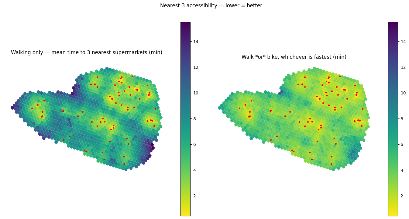
12. Cross-modal accessibility (time domain): nearest-k via fastest mode¶
With walk and bike costs both available, the simplest cross-modal accessibility metric is “what’s the mean time to the 3 nearest supermarkets, if a traveller always picks whichever mode is fastest for each destination”. Walking wins the very short trips (no overhead); cycling wins the longer ones (speed dominates once the setup time has been amortised).
Why this needs in-loop aggregation across modes — and not a simple “average the per-mode nearest-k results” shortcut:
Computing per-mode nearest-k separately and combining double-counts supermarkets reachable by both modes and loses the “pick fastest” semantics entirely.
The right answer requires taking
min(walk_cost, bike_cost)for every OD pair before applying the nearest-k aggregator.
od_pairs.aggregate_across_modes does exactly that: it unions the per-mode OD pair sets per origin and applies the per-OD aggregator (here: elementwise min across modes, treating unreachable as inf).
[29]:
def fastest_mode_cost(stacked: np.ndarray) -> np.ndarray:
    """Per-OD elementwise min cost across modes.

    Stacked shape: `(n_modes, n_dests)`. NaN entries (mode-unreachable
    for that OD pair) are treated as inf so the min picks any
    reachable mode. Returns inf for OD pairs no mode can reach.
    """
    finite_stack = np.where(np.isnan(stacked), np.inf, stacked)
    return finite_stack.min(axis=0)


fastest_pairs, fastest_times = od_pairs.aggregate_across_modes(
    {'walk': (pairs_geo, times_geo),
     'bike': (bike_pairs_geo, bike_times_geo)},
    aggregator=fastest_mode_cost,
)
sm_weights_fastest = od_pairs.lookup_dest_column_geo(
    'supermarkets', fastest_pairs, cells, zones=zones,
)
acc_nk_fastest = accessibility.nearest_k(
    fastest_times, {'supermarkets': sm_weights_fastest},
    cell_to_zone, ks=[1, 3, 5],
)
acc_nk_fastest.head()
[29]:
| k | 1 | 3 | 5 |
|---|---|---|---|
| property | supermarkets | supermarkets | supermarkets |
| cell | |||
| 8a1fb4674017fff | 159.014526 | 246.606918 | 277.053131 |
| 8a1fb4671a77fff | 307.199951 | 338.753571 | 368.253357 |
| 8a1fb4671b17fff | 8.532490 | 158.272385 | 223.994537 |
| 8a1fb467426ffff | 181.113174 | 215.821106 | 266.438721 |
| 8a1fb4675327fff | 318.934265 | 332.472870 | 340.419556 |
Visualise: walking-only nearest-3 (from §8) vs cross-modal “fastest- mode” nearest-3, on a shared scale (minutes, lower = better). The bike-helps map (right) should be uniformly faster than walk-only (left); the gap reveals where cycling earns its overhead back.
[30]:
viz.plot_cell_values_comparison(
    cells,
    {'Walking only — mean time to 3 nearest supermarkets (min)':
         acc_nk[(3, 'supermarkets')] / 60,
     'Walk *or* bike, whichever is fastest (min)':
         acc_nk_fastest[(3, 'supermarkets')] / 60},
    suptitle='Nearest-3 accessibility — lower = better',
    cmap='viridis_r',
    overlays=[(supermarkets, {'color': 'red', 'markersize': 8})],
)
plt.show()
13. Utility-based accessibility & cross-modal logsum¶
Discrete-choice-style accessibility: define a per-mode utility function combining travel cost, per-edge route features, and endpoint features, then derive the canonical logsum accessibility from it. Cycling is the more interesting case (it carries a route-feature term for bike- friendliness from §11), so we lead with bike; walking, a simpler cost-only spec, follows. We then combine both modes into a single cross-modal logsum.
A linear utility per OD pair:
U_ij = constant
     + β_cost · cost_ij                       (routing weight)
     + Σ_f β_f · aggregated_f(i, j)            (route features)
     + Σ_o β_o · feature_o(i)                  (origin features)
     + Σ_d β_d · feature_d(j)                  (destination features)
13.1 Bike utility with a route-feature¶
U_bike = −7 − 0.7 · (t_bike / 60) + 0.7 · mean_bike_score_on_path
Constant −7: Alternative-specific constant. Non-trivial setup before any trip (walk to bike, unlock, helmet).
Time coefficient −0.7 / minute: time costs disutility, but less per minute than walking (−1, below). Cycling time is less unpleasant minute-for-minute.
Route-feature coefficient +1.0 on mean bike-friendliness score:
edge_bike_scorefrom §11 (1 = busy primary, 5 = cycleway), averaged along the realised route. Positive coefficient = bike-friendlier routes raise utility.
RouteFeature triggers tiered_path_aggregate internally — one routing pass returns both the cost and the per-OD-pair averaged bike score along the realised path.
[31]:
bike_utility = utility.Utility(
    constant=-7.0,
    cost_coefficient=-0.7 / 60.0,    # utils per second (= −0.7 per minute)
    route_features=[
        utility.RouteFeature(
            name='bike_score_avg',
            attribute=edge_bike_score,
            coefficient=0.7,
            aggregator='mean',
        ),
    ],
)
Step 1: compute the route-dependent utility components (β_cost · cost + Σ β_route · feature). Wraps tiered_path_aggregate internally so the routing pass is shared across the cost and all features.
[32]:
bike_route_u = utility.route_utility(bike_graph, bike_pairs, weight='bike_time_s', utility=bike_utility,
)
Step 2: add the constant + origin + destination components. This example has neither origin nor destination features in the utility (the destination “attractiveness” enters via the supermarket weight in the gravity step below), so this just adds the −4 constant.
[33]:
bike_full_u = utility.add_endpoint_utility(
    bike_route_u, bike_pairs, bike_utility, cells=cells,
)
Step 3: lift to geo-keyed form, then bake the per-cell bike origin overhead into the utility ODM via add_geo_overheads. Units already match (utils + utils) because we pre-multiply bike_overhead_s by β_cost, so no per-call overhead-conversion is needed.
[34]:
_, bike_full_u_geo = od_pairs.reindex_by_geo_unit(
    bike_pairs, bike_full_u, cells,
    cell_node_column='bike_node_id',
    zones=zones, zone_node_column='bike_node_id',
    r_cells=R_CELLS, r_medium=R_MEDIUM, r_zones=R_ZONES,
)
cells['bike_util_overhead'] = bike_utility.cost_coefficient * cells['bike_overhead_s']
bike_full_u_geo = overhead.add_geo_overheads(
    bike_full_u_geo, bike_pairs_geo,
    origin_cell=cells['bike_util_overhead'],
    cell_to_zone=cells['zone_id'],
)
13.2 Walking utility (cost-only)¶
U_walk = −3 − 1 · (t_walk / 60)
Smaller constant (−3 vs −7) reflects walking’s lower setup cost; stronger time coefficient (−1 vs −0.7 per minute) reflects that a minute of walking is more onerous than a minute of cycling. No route feature → the pipeline is identical to bike but skips the per-edge aggregation pass.
[35]:
walking_utility = utility.Utility(
    constant=-3.0,
    cost_coefficient=-1.0 / 60.0,
)
route_u = utility.route_utility(graph, pairs, weight='walk_time_s', utility=walking_utility,
)
full_u = utility.add_endpoint_utility(route_u, pairs, walking_utility, cells=cells)
_, full_u_geo = od_pairs.reindex_by_geo_unit(
    pairs, full_u, cells,
    cell_node_column='node_id',
    zones=zones, zone_node_column='node_id',
    r_cells=R_CELLS, r_medium=R_MEDIUM, r_zones=R_ZONES,
)
cells['util_overhead'] = walking_utility.cost_coefficient * cells['walk_overhead_s']
full_u_geo = overhead.add_geo_overheads(
    full_u_geo, pairs_geo,
    origin_cell=cells['util_overhead'],
    cell_to_zone=cells['zone_id'],
)
13.3 Per-mode logsum accessibility¶
Gravity-on-utility with the exp decay = expected sum of attractiveness across destinations, weighted by exp(utility). Taking the log of that sum gives the canonical logsum accessibility — the discrete-choice expected utility from the choice set.
Logsum is in the same units as utility (utils). It can be negative when the accessible attractiveness is low — that’s expected for cells far from any supermarket or facing long travel times. Less negative = better access. When no destinations are reachable, the gravity sum is 0 and log(0) = -inf; viz treats these as missing.
[36]:
# Custom decay: gravity expects `exp(-β · cost)`, but utility is "more = better"
# (not a cost). Plain `np.exp` applied to utility gives the correct exp(U).
exp_utility_decay = accessibility.Decay('exp_u', np.exp)

# Walk-only logsum.
gravity_u_walk = accessibility.gravity(
    full_u_geo, {'supermarkets': sm_weights}, cell_to_zone, exp_utility_decay,
)
walk_logsum = np.log(gravity_u_walk[('exp_u', 'supermarkets')]).rename('walk_logsum')

# Bike-only logsum. Destination weights aligned to bike_pairs_geo: same cells
# as the walk weights, but the per-origin reachable sets differ.
sm_weights_bike = od_pairs.lookup_dest_column_geo(
    'supermarkets', bike_pairs_geo, cells, zones=zones,
)
gravity_u_bike = accessibility.gravity(
    bike_full_u_geo, {'supermarkets': sm_weights_bike}, cell_to_zone,
    exp_utility_decay,
)
bike_logsum = np.log(gravity_u_bike[('exp_u', 'supermarkets')]).rename('bike_logsum')
13.4 Cross-modal logsum (walk + bike, utility domain)¶
The canonical cross-modal logsum accessibility:
A_i = ln Σ_j W_j Σ_m exp(U_ijm)
Combine the per-mode utility ODMs into a single combined ODM via aggregate_across_modes with a custom utility-domain logsum aggregator, then apply gravity-on-utility + log.
Note on equivalence with the per-mode shortcut. Unlike the cross-modal nearest-k in §12 (where the in-loop min was load-bearing), the gravity-on-utility logsum is algebraically ln(Σ_m G_im) where G_im = Σ_j W_j · exp(U_ijm) is the per-mode gravity-on-utility — i.e. log(exp(walk_logsum) + exp(bike_logsum)) gives the same answer (a sum-order swap). The in-loop pattern below is here for API consistency with §12, dest-set-union handling, and skipping an exp → log → exp → log
round-trip. For cumulative-opportunity or nearest-k cross-modal accessibility the in-loop aggregation is the only mathematically correct path.
[37]:
def logsum_utility(stacked: np.ndarray) -> np.ndarray:
    """Cross-modal logsum in *utility* space (more = better).

    Stacked shape: `(n_modes, n_dests)`. Per OD pair, returns
    `ln Σ_m exp(U_ijm)` — the expected-max-utility across modes.
    NaN entries (mode unreachable for that OD pair) contribute 0 to the sum.
    """
    exp_terms = np.exp(stacked)
    exp_terms = np.where(np.isnan(exp_terms), 0.0, exp_terms)
    sum_exp = exp_terms.sum(axis=0)
    with np.errstate(divide='ignore'):
        return np.log(sum_exp)


combined_u_pairs, combined_u = od_pairs.aggregate_across_modes(
    {'walk': (pairs_geo, full_u_geo),
     'bike': (bike_pairs_geo, bike_full_u_geo)},
    aggregator=logsum_utility,
)

# Destination weights aligned to the UNION dest set across modes.
sm_weights_combined = od_pairs.lookup_dest_column_geo(
    'supermarkets', combined_u_pairs, cells, zones=zones,
)
gravity_combined = accessibility.gravity(
    combined_u, {'supermarkets': sm_weights_combined}, cell_to_zone,
    exp_utility_decay,
)
cross_modal_logsum = np.log(
    gravity_combined[('exp_u', 'supermarkets')]
).rename('cross_modal_logsum')
Side-by-side: walk-only, bike-only, and cross-modal walk-or-bike logsum, on a shared colour scale. Cells where no mode reaches any supermarket appear as missing.
[38]:
viz.plot_cell_values_comparison(
    cells,
    {'Walking only': walk_logsum,
     'Cycling only': bike_logsum,
     'Cross-modal (walk + bike)': cross_modal_logsum},
    suptitle='Logsum accessibility to supermarkets — less negative = better',
    overlays=[(supermarkets,
               {'color': 'red', 'markersize': 10, 'edgecolor': 'black'})],
)
plt.show()
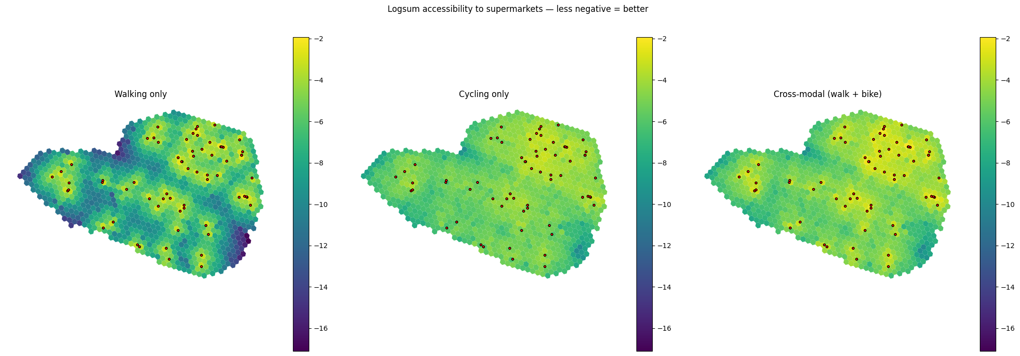
The cross-modal map is uniformly less negative (better) than either single-mode map — adding a second mode can only expand reachability. The gap between walking-only and cross-modal is largest in cells far from any supermarket: walking sees long travel times (very negative utility, very small contribution to the gravity sum), but cycling brings them within practical reach. In dense central cells with many walkable supermarkets, the walking utility already dominates the modal sum and the cross-modal addition is small. In addition, we see the cycling infrastructure quality (mean bike score on routes) take effect: cycling utility, and therefore combined utility, is strongest and most homogeneous in the northeastern part of the city, where the mean bike-friendliness along routes was highest.
Architectural notes:
Each mode has its own graph, its own node IDs, its own edge attributes, and its own snapping. Alignment happens only at the geo-unit (cell / zone) level via
TieredODGeoPairs.Per-mode origin overhead is baked into the per-mode utility ODM before aggregation, so the cross-modal logsum sees the right mode-specific first-mile cost (walking at 1.4 m/s vs cycling with a 30-second unlock setup).
aggregate_across_modesunions the per-origin dest sets across modes and fills missing entries withinf(mode-unreachable). For our example, walk and bike cover roughly the same Central Paris cells, but at country scale this matters — different modes naturally reach different sub-graphs.Destination-side overheads (last-mile, also mode-specific) are NOT baked into the utility ODMs in this walkthrough. A production analysis would add them via
add_geo_overheads(dest_cell=..., dest_zone=...)on each per-mode utility ODM before aggregation, using mode-specific utils-per-second conversions.