Multi-modal accessibility — extended example¶

Default scope: Bern + 40 km (10 km AOI buffer + 30 km dest buffer). Change LOCATION_LABEL and the crop constants below to retarget plots; the underlying data is whatever prepare/1_download produced (driven by SEED_LOCATION there).

Tutorial-scope accessibility analysis across three modes (walk, bike, car) on real OSM data, with published-paper edge-weight coefficients applied inline. One representative variant per mode for clarity. Ends with a cross-modal logsum that combines all three modes into one accessibility surface.

Inputs (all from prepare/):

3 consolidated networks (walk_graph, bike_graph, car_graph) carrying per-edge features from prep: speed_kph, density_norm, elev_gain, elev_loss, is_4way, is_traffic_signal. Edge travel times are computed inline in section 2 below by applying published coefficients to these features.
H3 cells (res 10) + zones (res 8) with population, employment_*, poi_* columns, plus pre-snapped node_id_{walk,bike,car} / snap_dist_* from prepare/3_unit_mapping.

Three destinations, picked to span the temporal-decay spectrum:

Destination	Column	Decay profile
Jobs (FTE)	`employment_total`	medium (commute)
Grocery shopping	`poi_errands_groceries`	sharp (frequent)
Hiking POIs	`poi_leisure_hiking`	slow (destination)

Three modes (one published variant each):

Mode	Edge attribute	Distance mask
walk	`walk_time_s`	< 5 km
bike (regular)	`bike_time_s`	< 25 km
car (peak)	`car_time_s_peak`	none

[1]:

import warnings
from pathlib import Path

import geopandas as gpd
import matplotlib.pyplot as plt
import numpy as np
import osmnx as ox
import pandas as pd

from aperta import (
    accessibility,
    geo_processing,
    network_processing,
    od_pairs,
    overhead,
    routing,
    routing_prep,
    visualization as viz,
)

warnings.filterwarnings("ignore", category=FutureWarning)
warnings.filterwarnings("ignore", category=UserWarning, module="geopandas")

PREPARED_DIR = Path("data/prepared")
CRS_METRIC = "EPSG:2056"

# === Plot retargeting knobs =================================================
# Keep in sync with `SEED_LOCATION` / `LOCATION_LABEL` in `prepare/1_download.py`.
#   - CITY_NAME: source of the city-shape outline in §9/12/13, fetched
#     unsmoothed from OSM (preserves the actual municipal boundary).
#   - CITY_CROP_*: square crop window each results panel renders into —
#     centred on `CITY_CROP_CENTER_XY`, `CITY_CROP_HALF_M` wide on each
#     side. The polygon extends beyond the crop on the western side;
#     that's fine, the crop trims it visually at the panel edge.
#   - NEIGHBORHOOD_*: building-level deep-zoom in §14.
LOCATION_LABEL = "Bern"
CITY_NAME = "Bern, Switzerland"
# Viewport east + north of station so the city silhouette sits in the
# lower-left of the panel (Bern extends NE → SW; this framing keeps
# the silhouette centred visually while showing more open countryside
# to the NE).
CITY_CROP_CENTER_XY = (2_600_800, 1_200_400)
CITY_CROP_HALF_M = 3_750  # approx. 7.5x7.5 km square window
NEIGHBORHOOD_CENTER_XY = (2_600_000, 1_199_600)  # LV95; central Bern (Bundeshaus)
NEIGHBORHOOD_HALF_M = 700  # 1.4 × 1.4 km window
# ============================================================================

Model coefficients and parameters¶

Lifted here for one-stop tuning. Display labels (mode / destination names) and figure-specific layout knobs stay near the sections that use them.

[2]:

# === Routing ================================================================
# Per-mode OD-tier radii (CRS-units, metres). Faster modes reach further
# → larger `r_zones`. cells_to_cells handles close pairs at full cell
# resolution; zones aggregate far destinations.
TIER_CUTOFFS = {
    "walk": dict(r_cells=1_500.0, r_medium=2_500.0, r_zones=5_000.0),
    "bike": dict(r_cells=1_500.0, r_medium=7_500.0, r_zones=25_000.0),
    "car": dict(r_cells=1_500.0, r_medium=10_000.0, r_zones=100_000.0),
}
# Per-mode route-time floor applied BEFORE overhead is added — both
# in §7 (for §8 nearest-k) and §12 (for utility logsum). Reflects the
# minimum sensible node-to-node trip cost, a trade-off accepted because
# consolidated networks lack nodes mid-edge: cells whose centroid snaps
# to the same network node have route(snap_A, snap_B) = 0, regardless
# of how far apart the centroids actually are. Without this floor,
# gravity-based metrics (logsum) get visible "islands" at high-multi-cell
# snap-nodes where weight aggregates and exp(-β·0) maxes out.
#
# Per-mode values reflect network density: walk is dense (~1.5 cells/
# snap-node avg → 60 s floor catches the rare snap-coincidence cases);
# bike is intermediate but residential streets still share snap-nodes;
# car is sparsest (~4.8 cells/snap-node avg, max 352 cells at one node
# in Bern, 2k+ aggregated jobs) so a more aggressive floor is needed.
# Cars also rarely make sub-2-min trips in practice — the floor matches
# behavioural reality.
MIN_ROUTE_S = {
    "walk": 60.0,
    "bike_regular": 60.0,
    "car_peak": 60.0,
}

# === Trip overhead (first/last-mile, per mode) ==============================
# overhead_s = constant + density × density_norm + snap_dist_<mode> / speed
# `constant` + `density` from Miotti et al. (Transportation, 20XX);
# `snap_dist_s_per_m` added to penalise cells far from the network
# (avoids artificial bright spots from cells right ON the network).
WALK_SPEED_MS = 1.4  # ~5 km/h
BIKE_SPEED_MS = 5.0  # ~18 km/h, matches the bike-graph base speed
CAR_FIRST_MILE_MS = 5.0  # parking-zone speed, NOT the driving speed
OVERHEAD_COEF = {
    "walk": {"const": 50, "density": 0, "snap_dist_s_per_m": 1 / WALK_SPEED_MS},
    "bike_regular": {"const": 70, "density": 50, "snap_dist_s_per_m": 1 / BIKE_SPEED_MS},
    "car_peak": {"const": 50, "density": 130, "snap_dist_s_per_m": 1 / CAR_FIRST_MILE_MS},
}

# === Utility coefficients (per-mode discrete-choice spec) ===================
# U_ijm = β_asc
#       + β_time      · t_min                       (linear time, per min)
#       + β_density   · mean(density_norm) along route
#       + β_bike_score· mean(bike_score)   along route
# `t_min` is the total cell-to-cell time including per-cell overhead
# (computed in §12 from route cost + 2 × `overhead.linear_per_cell_overhead`),
# so it's always > 0 — `ln(t_min)` doesn't need a floor here.
# Approximations informed by an ongoing project; placeholders pending a
# public reference.

UTILITY_COEF = {
    "walk": {
        "asc": 0.0,
        "time": -1.0,
        "density": 0.0,
        "bike_score": 0.5
    },
    "bike_regular": {
        "asc": -4.0,
        "time": -0.6,
        "density": -0.2,
        "bike_score": 1.5,
    },
    "car_peak": {
        "asc": -6.0,
        "time": -0.4,
        "density": -0.6,
        "bike_score": 0.0
    },
}

# === Accessibility metrics ==================================================
# Per-destination K for time-based nearest-k (§8). Destination-type
# specific (not mode-specific): groceries are picked from the nearest
# few stores, employment from a much broader effective choice set.
# Output: mean travel time over the first K weight-units.
DEST_K = {
    "employment_total": 5000,
    "poi_errands_groceries": 3,
    "poi_leisure_hiking": 10,
}
# Per-destination nest scale θ for utility logsum (§12/§13). Larger θ →
# broader decay (many destinations contribute); smaller θ → sharper
# decay (nearest dominate). Logsum = θ · ln Σ_j exp(U_ij/θ).
DEST_NEST_SCALE = {
    "employment_total": 6.0,
    "poi_errands_groceries": 1.0,
    "poi_leisure_hiking": 3.0,
}

# === Example route knobs (§11 path-aggregation showcase) ====================
# §11 picks the cell whose centroid is nearest to EXAMPLE_ORIGIN_XY as
# the example origin, then renders the K nearest grocery routes from
# it on top of the per-cell aggregation map.
EXAMPLE_ORIGIN_XY = (2_600_800, 1_199_800)  # in old town
EXAMPLE_K_ROUTES = 30
# §11 aggregation: route to the nearest K grocery stores from each origin
# cell, then take the mean feature along those routes. "Stores", not
# "cells" — destination cells with multiple groceries count proportionally
# (and may be partially counted to hit exactly K).
NEAREST_K_GROCERIES = 10
# ============================================================================

1. Load networks + geo units¶

[3]:

walk_graph = network_processing.load_consolidated_graphml(PREPARED_DIR / "walk_graph.graphml")
bike_graph = network_processing.load_consolidated_graphml(PREPARED_DIR / "bike_graph.graphml")
car_graph = network_processing.load_consolidated_graphml(PREPARED_DIR / "car_graph.graphml")

# `ox.load_graphml` returns edge attributes as strings (except those
# registered in `CONSOLIDATED_EDGE_DTYPES`). Cast the features we use
# in the edge-weight formula below back to float.
FEATURE_COLS = (
    "length",
    "speed_kph",
    "density_norm",
    "elev_gain",
    "elev_loss",
    "is_t_junction",
    "is_4way",
    "is_traffic_signal",
)
for g in (walk_graph, bike_graph, car_graph):
    for _, _, d in g.edges(data=True):
        for c in FEATURE_COLS:
            if c in d:
                d[c] = float(d[c])

print(f"Walk: {walk_graph.number_of_nodes():>7,} nodes / {walk_graph.number_of_edges():>7,} edges")
print(f"Bike: {bike_graph.number_of_nodes():>7,} nodes / {bike_graph.number_of_edges():>7,} edges")
print(f"Car:  {car_graph.number_of_nodes():>7,} nodes / {car_graph.number_of_edges():>7,} edges")

# Apply mode-aware preparation: undirected + largest-CC snap for walk
# and bike, directed + largest-SCC snap for car. Each call also tags
# mode-non-traversable edges (motorway/trunk for walk) as cost-excluded
# via a per-edge boolean attribute named on `prepared.cost_excluded_flag`.
walk_prepared = routing_prep.prepare_network(walk_graph, "walk")
bike_prepared = routing_prep.prepare_network(bike_graph, "bike")
car_prepared = routing_prep.prepare_network(car_graph, "car")
walk_graph = walk_prepared.graph
bike_graph = bike_prepared.graph
car_graph = car_prepared.graph

Walk: 230,031 nodes / 677,181 edges
Bike: 208,164 nodes / 558,734 edges
Car:   60,892 nodes / 144,694 edges

[4]:

cells = gpd.read_file(PREPARED_DIR / "cells.gpkg").set_index("cell_id")
zones = gpd.read_file(PREPARED_DIR / "zones.gpkg").set_index("zone_id")

print(
    f"Cells: {len(cells):>6,}  (Σ pop {cells['population'].sum():>10,.0f}, "
    f"Σ jobs {cells['employment_total'].sum():>10,.0f})"
)
print(f"Zones: {len(zones):>6,}")

DESTINATIONS = ["employment_total", "poi_errands_groceries", "poi_leisure_hiking"]
for d in DESTINATIONS:
    print(f"  Σ {d:25s}: {cells[d].sum():>10,.0f}")

Cells: 142,209  (Σ pop  1,551,024, Σ jobs    722,153)
Zones:  8,903
  Σ employment_total         :    722,153
  Σ poi_errands_groceries    :      2,123
  Σ poi_leisure_hiking       :      7,590

[5]:

# Origin / destination split — origins are only cells inside the AOI
# (seed + 10 km from `prepare/1_download`), but every cell in the dest
# polygon (AOI + 30 km) remains a valid destination. This dramatically
# cuts routing cost: each Dijkstra is one-to-many, so the cost scales
# with origin count, not destination count.
aoi_polygon = gpd.read_file(PREPARED_DIR / "aoi_polygon.gpkg").geometry.iloc[0]
ORIG_MASK = cells.geometry.centroid.within(aoi_polygon)
print(
    f"\nOrigin cells: {ORIG_MASK.sum():,} of {len(cells):,} "
    f"({100 * ORIG_MASK.mean():.1f}%) inside AOI; "
    f"all {len(cells):,} remain valid destinations."
)


Origin cells: 20,900 of 142,209 (14.7%) inside AOI; all 142,209 remain valid destinations.

[6]:

# City polygon (for the silhouette outline in §9/12/13) and POI points
# (for overlays on supermarket / hiking-POI panels). The polygon comes
# from OSM via `osmnx.geocode_to_gdf`, unsmoothed — the actual municipal
# boundary. The square crop window (see `CITY_CROP_*` above) trims the
# polygon visually at panel edges; the western strip is cut off there.
import _figures as figures  # noqa: E402  — project-local plot helpers

CITY_POLYGON = figures.fetch_city_polygon(
    CITY_NAME,
    target_crs=CRS_METRIC,
    smooth=False,
)
pois = gpd.read_file(PREPARED_DIR / "pois.gpkg")
print(f"{CITY_NAME}: polygon area {CITY_POLYGON.area / 1e6:.1f} km²; {len(pois):,} POIs loaded.")

Bern, Switzerland: polygon area 51.6 km²; 11,219 POIs loaded.

2. Apply published edge-weight coefficients → per-edge travel times¶

Coefficients from Miotti et al., Transportation, 20XX, hardcoded inline for visibility. One representative variant per mode (walk, regular bike, peak car).

Formula — per directed edge u → v of length L m:

effective_kph = max(base_speed_kph · (1 + β_density · density_norm), floor_kph)
duration_s    = L / (effective_kph / 3.6)
              + α_up   · elev_gain                     (m climbed u→v)
              + α_down · elev_loss                     (m descended u→v)
              + β_intersection_4 · is_4way             (∈ {0, 0.5, 1})
              + β_traffic_signal · is_traffic_signal   (∈ {0, 0.5, 1})

Bike additionally caps the downhill speed at 50 km/h — without it, the negative α_down makes short steep descents produce negative-duration edges (Dijkstra silently churns).

The simplifications vs the paper (also documented in the “what this notebook does NOT do” footer):

One variant per mode (no e-bike, no peak/night car).
β_intersection (3-way) absent — published 9-row schema only has the 4-way coefficient.

[7]:

def apply_edge_times(
    graph,
    attr_name: str,
    *,
    base_speed_kph: float | None,
    alpha_up: float,
    alpha_down: float,
    beta_density: float,
    beta_intersection_4: float,
    beta_traffic_signal: float,
    floor_kph: float = 1.0,
    max_downhill_kph: float | None = None,
    cost_excluded_flag: str | None = None,
) -> None:
    """Apply the published-coefficient formula and write to `attr_name`.

    `base_speed_kph=None` means "read per-edge `speed_kph`" (used for car).
    `max_downhill_kph` caps the implied speed on edges where the slope
    bonus would otherwise drive duration negative (used for bike).
    `cost_excluded_flag`, if given, names a per-edge bool attribute on
    `graph` (typically `prepared.cost_excluded_flag`); flagged edges
    get `attr_name = inf` instead of the formula — used to mask
    mode-non-traversable edges marked by `prepare_network`.
    """
    min_dur_per_m = None if max_downhill_kph is None else 1.0 / (max_downhill_kph / 3.6)
    for _, _, _, data in graph.edges(keys=True, data=True):
        if cost_excluded_flag is not None and data.get(cost_excluded_flag, False):
            data[attr_name] = float("inf")
            continue
        base_kph = data["speed_kph"] if base_speed_kph is None else base_speed_kph
        effective_kph = max(base_kph * (1 + beta_density * data["density_norm"]), floor_kph)
        base_dur = data["length"] / (effective_kph / 3.6)
        slope_pen = alpha_up * data["elev_gain"] + alpha_down * data["elev_loss"]
        intersection_pen = (
            beta_intersection_4 * data["is_4way"]
            + beta_traffic_signal * data["is_traffic_signal"]
        )
        total = base_dur + slope_pen + intersection_pen
        if min_dur_per_m is not None:
            total = max(total, data["length"] * min_dur_per_m)
        data[attr_name] = total


# Walk — slow, no density slowdown, intersection penalties zero in the
# paper (pedestrians don't wait at signals in the same way). Motorway /
# trunk edges flagged by `prepare_network` get cost = ∞ via
# `cost_excluded_flag`.
apply_edge_times(
    walk_graph,
    "walk_time_s",
    base_speed_kph=5.0,
    alpha_up=2.4,
    alpha_down=0.1,
    beta_density=0.0,
    beta_intersection_4=0.0,
    beta_traffic_signal=0.0,
    cost_excluded_flag=walk_prepared.cost_excluded_flag,
)

# Bike (regular) — steeper climbs, slight downhill bonus (capped at
# 50 km/h to avoid negative durations on steep descents). Bike defaults
# have no excluded tags, so the flag pass-through is a no-op here.
apply_edge_times(
    bike_graph,
    "bike_time_s",
    base_speed_kph=18.0,
    alpha_up=3.1,
    alpha_down=-0.3,
    beta_density=0.0,
    beta_intersection_4=7.0,
    beta_traffic_signal=1.0,
    max_downhill_kph=50.0,
    cost_excluded_flag=bike_prepared.cost_excluded_flag,
)

# Car (peak) — per-edge baseline from OSM `maxspeed`, density
# slowdown (urban friction), intersection + signal penalties.
apply_edge_times(
    car_graph,
    "car_time_s_peak",
    base_speed_kph=None,
    alpha_up=0.0,
    alpha_down=0.0,
    beta_density=-0.20,
    beta_intersection_4=6.0,
    beta_traffic_signal=10.0,
    floor_kph=15.0,
    cost_excluded_flag=car_prepared.cost_excluded_flag,
)

for label, graph, attr in [
    ("walk", walk_graph, "walk_time_s"),
    ("bike", bike_graph, "bike_time_s"),
    ("car", car_graph, "car_time_s_peak"),
]:
    times = np.array([d[attr] for _, _, d in graph.edges(data=True)])
    lengths = np.array([d["length"] for _, _, d in graph.edges(data=True)])
    implied_kph = (lengths / times) * 3.6
    print(
        f"  {label:5s} {attr:20s}: median edge time {np.median(times):>6.1f} s, "
        f"implied speed {np.median(implied_kph):.1f} km/h"
    )

  walk  walk_time_s         : median edge time   75.5 s, implied speed 4.9 km/h
  bike  bike_time_s         : median edge time   26.4 s, implied speed 16.2 km/h
  car   car_time_s_peak     : median edge time   12.7 s, implied speed 40.2 km/h

3. Build tiered OD pairs — per network¶

Per-mode tier cutoffs (Euclidean metres). The three tiers split each origin’s destination universe into:

cells_to_cells (dest distance < r_cells): per-cell origin and dest — the highest-precision tier, kept small to bound storage.
cells_to_zones (r_cells ≤ d < r_medium): per-cell origin, zone-aggregated dest — preserves the origin precision where the cell-to-cell pair count would explode but the relative cost of a specific dest cell within its zone is still meaningful.
zones_to_zones (r_medium ≤ d < r_zones): zone-aggregated both sides — coarse but cheap, sized for long-haul.

Per-mode reasoning: faster modes reach further, so r_zones scales with mode speed. Walk barely needs a far tier (the 5 km mask in section 4 drops anything longer anyway); car runs all the way to the dest-polygon edge. The shared geo-unit grid (same cells / zones) means the per-mode ODMs can be lifted to TieredODGeoPairs and fed to od_pairs.aggregate_across_modes for the cross-modal logsum at the bottom of this notebook.

[8]:

# `TIER_CUTOFFS` defined at the top of this notebook.
PAIRS = {}
for label, graph in [("walk", walk_graph), ("bike", bike_graph), ("car", car_graph)]:
    pairs = od_pairs.get_pairs(
        cells,
        node_column=f"node_id_{label}",
        zones=zones,
        orig_cells=ORIG_MASK,
        **TIER_CUTOFFS[label],
    )
    PAIRS[label] = pairs
    print(f"  {label:5s} {pairs}")

  walk  TieredODNodePairs(cells_to_cells: 17,333 orig → 2,595,152 dest; cells_to_zones: 17,333 orig → 419,559 dest; zones_to_zones: 1,107 orig → 92,394 dest)
  bike  TieredODNodePairs(cells_to_cells: 16,823 orig → 2,426,090 dest; cells_to_zones: 16,823 orig → 4,093,355 dest; zones_to_zones: 1,107 orig → 2,715,683 dest)
  car   TieredODNodePairs(cells_to_cells: 9,369 orig → 931,515 dest; cells_to_zones: 9,369 orig → 4,013,001 dest; zones_to_zones: 1,010 orig → 6,802,566 dest)

4. Distance-based masks — drop unrealistic walk / bike trips¶

Walking 27 km to work doesn’t happen — masking out long pairs before routing skips Dijkstra for them entirely. The walk graph is huge (290k nodes); the mask cuts routing time roughly in proportion to the pairs dropped.

[9]:

def make_distance_mask(pairs, graph, cutoff_m: float):
    """Build a TieredODNodePairs of bools from euclidean node distances."""
    nodes_xy = pd.DataFrame.from_dict(
        {n: (float(graph.nodes[n]["x"]), float(graph.nodes[n]["y"])) for n in graph.nodes},
        orient="index",
        columns=["x", "y"],
    )
    dists = od_pairs.get_euclidean_dists(nodes_xy, pairs)
    return od_pairs.make_mask(dists, lambda d: d < cutoff_m)


MASKS = {
    "walk": make_distance_mask(PAIRS["walk"], walk_graph, cutoff_m=5_000),
    "bike": make_distance_mask(PAIRS["bike"], bike_graph, cutoff_m=25_000),
    # car: no mask (any pair is potentially reachable in reasonable time).
}


def _mask_kept_pct(mask):
    tot = kept = 0
    for tier_name in ("cells_to_cells", "cells_to_zones", "zones_to_zones"):
        tier = getattr(mask, tier_name)
        if tier is None:
            continue
        for arr in tier.values():
            tot += arr.size
            kept += int(arr.sum())
    return 100 * kept / tot if tot else 0.0


print(f"  walk mask: keeps {_mask_kept_pct(MASKS['walk']):.1f}% of pairs")
print(f"  bike mask: keeps {_mask_kept_pct(MASKS['bike']):.1f}% of pairs")

  walk mask: keeps 99.9% of pairs
  bike mask: keeps 99.9% of pairs

5. Travel-cost ODMs — one per (mode, variant)¶

routing.tiered_path_costs runs Dijkstra per origin, summing the specified edge attribute along each shortest path. Pairs with a False mask entry are skipped (the cost ODM stores inf for them, which gravity / cumulative metrics treat as unreachable).

cutoff= truncates each per-origin Dijkstra once it crosses the given network-cost threshold. Picked per mode as a comfortable upper bound on plausible trip duration — destinations beyond it return inf and gravity / cumulative metrics drop them. Large speed-up on country-scale graphs without changing any answer.

[10]:

ROUTING_PLAN = [
    # (label,             graph,      pairs,         mask,           edge attr,            cutoff_s)
    ("walk", walk_graph, PAIRS["walk"], MASKS["walk"], "walk_time_s", 60 * 60),
    ("bike_regular", bike_graph, PAIRS["bike"], MASKS["bike"], "bike_time_s", 60 * 60),
    ("car_peak", car_graph, PAIRS["car"], None, "car_time_s_peak", 120 * 60),
]
# This showcase uses one representative variant per mode. The published
# paper has more (e-bike 25/45, car peak/night) — see projects/lumos/ for
# the production pipeline that exercises all of them with per-scenario
# coefficient tables.
import time

COSTS = {}
ROUTING_TIMES = {}
for label, graph, pairs, mask, weight, cutoff_s in ROUTING_PLAN:
    t0 = time.perf_counter()
    COSTS[label] = routing.tiered_path_costs(
        pairs,
        graph,
        weight=weight,
        mask=mask,
        cutoff=cutoff_s,
    )
    ROUTING_TIMES[label] = time.perf_counter() - t0
    print(f"  Routed {label:14s} ({weight:22s}) in {ROUTING_TIMES[label]:>6.1f} s", flush=True)
print(f"\nTotal routing time: {sum(ROUTING_TIMES.values()):.1f} s")

  Routed walk           (walk_time_s           ) in   15.2 s
  Routed bike_regular   (bike_time_s           ) in   57.9 s
  Routed car_peak       (car_time_s_peak       ) in   79.0 s

Total routing time: 152.1 s

6. Lift to geo-keyed form + destination weights¶

Routing returns node-keyed cost ODMs. To get per-cell accessibility output and (later) cross-modal aggregation, lift each to a TieredODGeoPairs via reindex_by_geo_unit. Then build one destination-value ODM per (mode, destination) — needed because the per-mode destination universes differ (different masks → different pair sets).

[11]:

NETWORK_OF = {
    "walk": "walk",
    "bike_regular": "bike",
    "car_peak": "car",
}

# Per-network: reindex once, build destination-value ODMs once. Variants
# on the same network share these — only the *cost* ODM differs per
# variant.
REINDEXED = {}  # net_label -> (pairs_geo, {destination: dest_vals_geo})
for net_label in ("walk", "bike", "car"):
    node_col = f"node_id_{net_label}"
    pairs_geo, _ = od_pairs.reindex_by_geo_unit(
        PAIRS[net_label],
        PAIRS[net_label],
        cells,
        cell_node_column=node_col,
        zones=zones,
        zone_node_column=node_col,
        **TIER_CUTOFFS[net_label],
    )
    dest_vals = {
        d: od_pairs.dest_values_geo(d, pairs_geo, cells, zones=zones) for d in DESTINATIONS
    }
    REINDEXED[net_label] = (pairs_geo, dest_vals)

# Per-variant: lift the cost ODM into geo-space.
GEO_PAIRS = {}
GEO_COSTS = {}
for label, _, pairs, _, _, _ in ROUTING_PLAN:
    net_label = NETWORK_OF[label]
    node_col = f"node_id_{net_label}"
    pairs_geo, cost_geo = od_pairs.reindex_by_geo_unit(
        pairs,
        COSTS[label],
        cells,
        cell_node_column=node_col,
        zones=zones,
        zone_node_column=node_col,
        **TIER_CUTOFFS[net_label],
    )
    GEO_PAIRS[label] = pairs_geo
    GEO_COSTS[label] = cost_geo

CELL_TO_ZONE = cells["zone_id"].to_dict()

7. Trip overheads — origin + destination first/last-mile¶

Each trip carries fixed per-mode overheads that don’t depend on routing:

Constant per side: door-to-network time (e.g. 49 s for walking, 74 s for biking — getting out the bike, unlocking, etc., 52 s for cars — finding parking, walking to/from).
Density: denser cells are slower to enter / leave (parking, wayfinding). Uses sqrt((pop + employment_total per km²) / 10_000) aggregated over a 1 km radius. Walking is unaffected (coef = 0); cars are most affected (parking searches scale with density).

Coefficients from Miotti et al., Transportation, 20XX, hardcoded inline below for visibility. The published table also has a constant overhead_*_dist term times cell-centroid-to-network-node distance — we drop it here as a tutorial simplification (cells are small enough that snap distances barely move the total), but the production pipeline in projects/lumos/ uses the full per-mode value.

Overheads apply at every tier: at the c2c tier the per-cell overhead is added directly at both origin and destination; at the c2z and z2z tiers, add_geo_overheads auto-derives the per-zone overhead as the mean of the per-cell overheads over each zone’s constituent cells (controllable via zone_aggregator=). Without zone-tier overheads, z2z trips would carry zero overhead while c2c carries 2× cell overhead — making far-tier destinations artificially cheap and producing visible origin-zone outlines in nearest-k accessibility maps. cell_to_zone is what enables the auto-derivation; pass it whenever your costs include c2z or z2z tiers.

[12]:

# Per-cell density — shared across all modes. Same formula and radius as
# in `prepare/4_edge_weights`: sqrt of (pop+emp / km² within 1 km, then
# normalised by 10_000).
cells["pop_plus_emp"] = cells["population"] + cells["employment_total"]
cells_centroids_gdf = cells.set_geometry(cells.geometry.centroid)
raw_per_m2 = geo_processing.cross_sum_within_radius(
    targets=cells_centroids_gdf,
    sources=cells_centroids_gdf,
    radius=1000.0,
    weight_column="pop_plus_emp",
    return_density=True,
)
cells["density_norm"] = np.sqrt(raw_per_m2 * 100.0)
print(
    f"Per-cell density_norm: median {cells['density_norm'].median():.3f}, "
    f"P95 {cells['density_norm'].quantile(0.95):.3f}, "
    f"max {cells['density_norm'].max():.3f}"
)

Per-cell density_norm: median 0.143, P95 0.578, max 1.451

[13]:

# `OVERHEAD_COEF` are defined at the top of this notebook. Bake the per-mode
# cell-tier overheads into each cost ODM.
GEO_COSTS_WITH_OVERHEAD = {}
for label, _, _, _, _, _ in ROUTING_PLAN:
    coef = OVERHEAD_COEF[label]
    net_label = NETWORK_OF[label]  # 'walk' / 'bike' / 'car'

    # Per-cell origin & destination overhead = constant
    #  + density × density_norm + snap_dist_s_per_m × snap_dist_<mode>.
    overhead_per_cell = overhead.linear_per_cell_overhead(
        cells,
        constant=coef["const"],
        feature_coefficients={
            "density_norm": coef["density"],
            f"snap_dist_{net_label}": coef["snap_dist_s_per_m"],
        },
    )

    # Overheads applied at every tier. `cell_to_zone` lets
    # `add_geo_overheads` auto-derive zone-tier overheads as the per-zone
    # mean of the per-cell values; without this, z2z OD pairs would carry
    # zero overhead while c2c carries 2× cell overhead, making far-tier
    # destinations artificially cheap and producing visible origin-zone
    # outlines in nearest-k accessibility maps.
    #
    # Route time floored at 60 s BEFORE adding overhead — kills the
    # snap-node-cluster boost (cell at snap node X gets near-zero cost
    # to other cells at X; cells one node over get a tiny route cost +
    # overhead; without flooring those two see very different totals
    # and the in-cluster cells appear as artificial bright islands).
    # After flooring, all sub-1-min routes look like 1-min routes,
    # then overhead is added uniformly per origin/dest cell.
    cost_floored = routing.floor_intrazonal_costs(GEO_COSTS[label], min_cost=MIN_ROUTE_S[label])
    GEO_COSTS_WITH_OVERHEAD[label] = overhead.add_geo_overheads(
        cost_floored,
        GEO_PAIRS[label],
        origin_cell=overhead_per_cell,
        dest_cell=overhead_per_cell,
        cell_to_zone=CELL_TO_ZONE,
    )
    print(
        f"  {label:14s}: per-cell overhead median {overhead_per_cell.median():>5.1f} s "
        f"(P95 {overhead_per_cell.quantile(0.95):>5.1f} s)"
    )

  walk          : per-cell overhead median  86.0 s (P95 141.2 s)
  bike_regular  : per-cell overhead median  90.3 s (P95 111.8 s)
  car_peak      : per-cell overhead median  83.5 s (P95 140.5 s)

8. Per-mode nearest-k accessibility (travel time, in minutes)¶

nearest_k answers: “how many minutes does it typically take to reach the K nearest opportunities of type X from this cell?” Direct, intuitive units (minutes); destination-type-specific K reflects how many opportunities of that type a typical traveller would consider substitutable.

K values are destination-type-specific (not mode-specific):

Destination	K	Rationale
Groceries (POIs)	3	People go to the nearest few
Hiking POIs	10	Some interchangeability, not too many
Employment (jobs)	5000	Many jobs are realistic options

Output: mean travel time (in minutes) over the first K weight-units. NaN where total reachable weight at an origin < K (e.g. walking can’t reach 5000 jobs from a peripheral cell — those cells show as missing on the map, an honest “out of range” answer).

Time floor on the route is set in §7 (60 s), so intrazonal / snap-node-coincidence pairs don’t get a free arbitrarily-fast contribution.

[14]:

# `DEST_K` defined at the top of this notebook.
ACC = {}  # (variant_label, destination) -> per-cell pd.Series (minutes)
for label, _, _, _, _, _ in ROUTING_PLAN:
    net_label = NETWORK_OF[label]
    _, dest_vals = REINDEXED[net_label]
    for d in DESTINATIONS:
        k = DEST_K[d]
        # `cost_mean` aggregator: mean cost over the first K weight-units.
        result = accessibility.nearest_k(
            GEO_COSTS_WITH_OVERHEAD[label],
            {d: dest_vals[d]},
            CELL_TO_ZONE,
            ks=[k],
        )
        # Cost is in seconds; convert to minutes for display.
        ACC[(label, d)] = result[(k, d)] / 60.0
        s = ACC[(label, d)].loc[ORIG_MASK].dropna()
        n_total = ORIG_MASK.sum()
        n_finite = len(s)
        print(
            f"  {label:14s} × {d:24s} (k={k:>4d}): "
            f"median {s.median():>5.1f} min  "
            f"P95 {s.quantile(0.95):>5.1f} min  "
            f"({n_finite:,}/{n_total:,} origins have ≥k reachable)"
        )

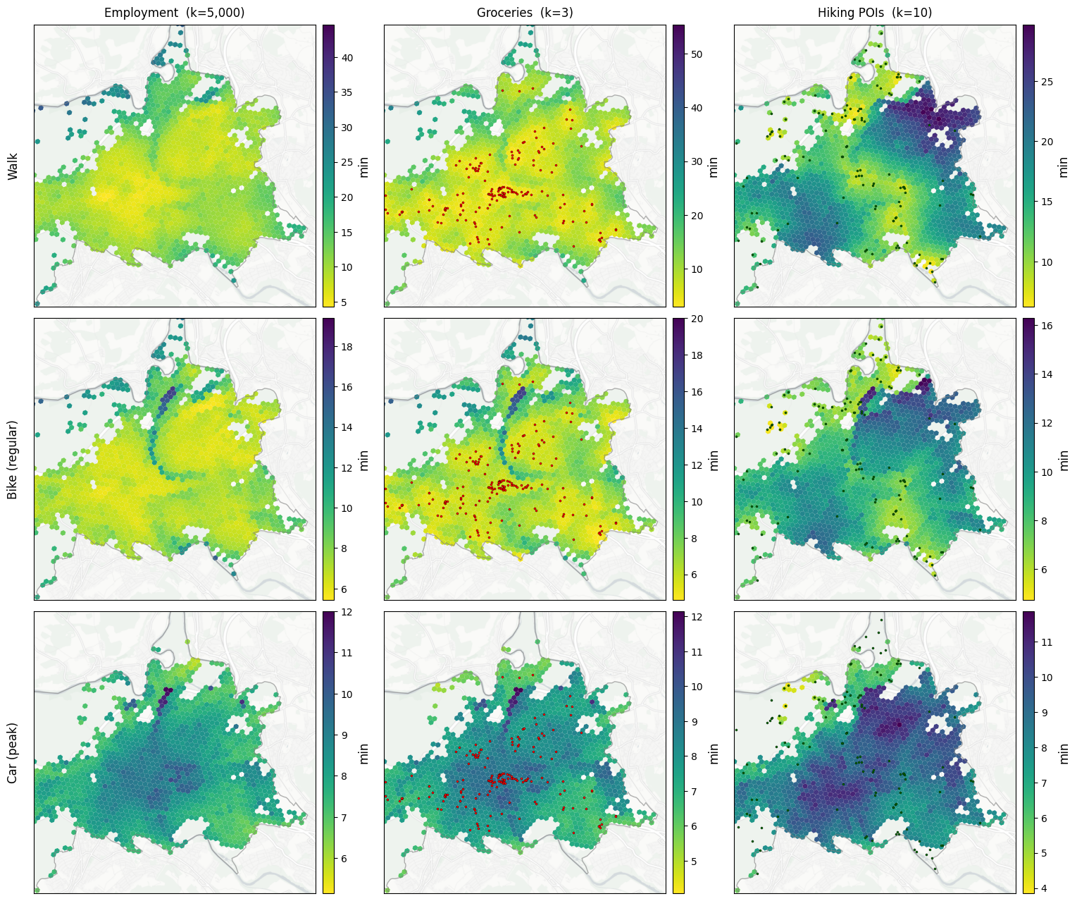
  walk           × employment_total         (k=5000): median  25.1 min  P95  46.7 min  (9,355/20,900 origins have ≥k reachable)
  walk           × poi_errands_groceries    (k=   3): median  20.0 min  P95  46.2 min  (19,843/20,900 origins have ≥k reachable)
  walk           × poi_leisure_hiking       (k=  10): median  20.2 min  P95  33.8 min  (20,782/20,900 origins have ≥k reachable)
  bike_regular   × employment_total         (k=5000): median  18.1 min  P95  30.3 min  (20,770/20,900 origins have ≥k reachable)
  bike_regular   × poi_errands_groceries    (k=   3): median   9.3 min  P95  19.0 min  (20,770/20,900 origins have ≥k reachable)
  bike_regular   × poi_leisure_hiking       (k=  10): median   9.2 min  P95  13.4 min  (20,770/20,900 origins have ≥k reachable)
  car_peak       × employment_total         (k=5000): median   8.2 min  P95  10.9 min  (17,132/20,900 origins have ≥k reachable)
  car_peak       × poi_errands_groceries    (k=   3): median   5.8 min  P95   8.4 min  (17,132/20,900 origins have ≥k reachable)
  car_peak       × poi_leisure_hiking       (k=  10): median   5.5 min  P95   8.8 min  (17,132/20,900 origins have ≥k reachable)

9. Per-mode maps (3 modes × 3 destinations) — nearest-k mean time¶

Each panel: mean travel time (minutes) to the nearest K opportunities of that destination type, where K is the destination-type-specific value from DEST_K. Colormap viridis_r so bright = short time = good access; dark = long time = poor access. Missing cells (white) are origins that can’t reach K of that destination type with this mode.

[15]:

ORIG_CELLS = cells.loc[ORIG_MASK]


def pois_overlay_for(destination: str):
    """POI overlay dict for `plot_city_focus`, keyed so default styling
    picks the right colour. None for non-POI destinations."""
    if destination == "poi_errands_groceries":
        return {"groceries": pois[pois["poi_errands_groceries"] > 0]}
    if destination == "poi_leisure_hiking":
        return {"hiking": pois[pois["poi_leisure_hiking"] > 0]}
    return None


# Display labels — used for shared row (mode) / column (destination)
# headers across §9, §12, §13. Per-panel titles are suppressed so the
# grid reads like a matrix.
MODE_LABELS = {
    "walk": "Walk",
    "bike_regular": "Bike (regular)",
    "car_peak": "Car (peak)",
}
DEST_LABELS = {
    "employment_total": f"Employment  (k={DEST_K['employment_total']:,})",
    "poi_errands_groceries": f"Groceries  (k={DEST_K['poi_errands_groceries']})",
    "poi_leisure_hiking": f"Hiking POIs  (k={DEST_K['poi_leisure_hiking']})",
}


fig, axes = plt.subplots(3, 3, figsize=(18.5, 16))
for row, (label, _, _, _, _, _) in enumerate(ROUTING_PLAN):
    for col, d in enumerate(DESTINATIONS):
        figures.plot_city_focus(
            axes[row, col],
            CITY_POLYGON,
            cells,
            ACC[(label, d)],
            pois=pois_overlay_for(d),
            crop_center_xy=CITY_CROP_CENTER_XY,
            crop_half_m=CITY_CROP_HALF_M,
            cmap="viridis_r",  # bright = short time = better access
            title="",
            label="min",
        )
        if row == 0:
            axes[row, col].set_title(DEST_LABELS[d], pad=8)
plt.subplots_adjust(wspace=0.13, hspace=0.04)
# Row labels via fig.text — using set_ylabel doesn't survive the
# divider-colorbar pattern reliably; figure-coord text always renders.
for row, (label, _, _, _, _, _) in enumerate(ROUTING_PLAN):
    pos = axes[row, 0].get_position()
    fig.text(
        pos.x0 - 0.012,
        (pos.y0 + pos.y1) / 2,
        MODE_LABELS[label],
        rotation=90,
        va="center",
        ha="center",
        fontsize=figures.LABEL_SIZE,
    )
figures.save_figure(fig, "accessibility_nearest_k_time")
plt.show()

Saved results/figures_highres/accessibility_nearest_k_time.png

../_images/examples_extended_accessibility_25_1.png

10. Per-mode utility specification¶

Section 8’s gravity accessibility weights destinations purely by trip time. That ignores everything we know about why trips happen — that the same trip time feels different on a quiet residential street vs a busy arterial, that long trips are increasingly painful per added minute, and that different modes have different inherent attractions (the alternative-specific constants).

A discrete-choice utility spec captures these per-mode (here m):

U_ijm = β_asc
      + β_time      · t_min                           (linear time, in min)
      + β_density   · mean(density_norm)  along route (per-edge density)
      + β_bike_score· mean(bike_score)    along route (per-edge quietness)

t_min is the total cell-to-cell travel time in minutes — (route_time + origin_overhead + dest_overhead) / 60, where overheads are the per-cell first/last-mile from §7. §12 computes it explicitly before plugging into the utility formula. Because overhead is always positive (≥ 49 s walk, ≥ 74 s bike, ≥ 52 s car, plus snap-distance), t_min > 0 always — the ln(t_min) term doesn’t need a floor.

bike_score is a per-edge quietness score from 1 (busy primary) to 5 (cycleway / pedestrian / quiet path), computed inline below from highway and cycleway* tags. High score is good for cycling and walking — quieter routes are pleasanter on foot too — but neutral for cars. density_norm is the same square-root per-edge density we routed on in §2.

[16]:

# Per-edge quietness score. 1 = motorway / busy primary; 5 = cycleway,
# footway, pedestrian path, or any edge with a dedicated bike track.
# Reads only OSM `highway` / `cycleway*` / `bicycle` tags so it works
# unchanged on all three networks.
def edge_bike_score(u, v, data) -> float:
    h = data.get("highway")
    if isinstance(h, list):
        h = h[0] if h else None
    if (
        h in ("cycleway", "footway", "pedestrian", "path", "living_street")
        or data.get("bicycle") == "designated"
    ):
        return 5.0
    rank = network_processing.OSM_HIGHWAY_RANKS.get(h, -1)
    if rank < 0:
        return 4.0  # service / track / unclassified — mid-good default
    # Higher OSM rank = busier road = worse.
    base = max(1, min(5, 6 - rank))
    cw = data.get("cycleway") or data.get("cycleway:left") or data.get("cycleway:right")
    if isinstance(cw, list):
        cw = cw[0] if cw else None
    if cw in ("track", "opposite_track"):
        bonus = 2
    elif cw:
        bonus = 1
    else:
        bonus = 0
    return float(min(5, base + bonus))


# `UTILITY_COEF` and `OVERHEAD_COEF` defined at the top of this notebook.


def floor_all_tiers(costs, min_cost: float):
    """Floor every finite cost in EVERY tier (cells_to_cells +
    cells_to_zones + zones_to_zones) at `min_cost`. Stricter than
    `routing.floor_intrazonal_costs`, which only touches cells_to_cells.

    Why we need this for §12 utility: an origin cell whose snap node
    coincides with a zone's snap node gets a 0-cost route to that
    zone's aggregated weight (potentially thousands of jobs). The
    library helper would leave that pair unfloored — and for car
    networks (sparse) the cells_to_zones + zones_to_zones tiers carry
    ~95% of the destination pairs, so flooring only cells_to_cells
    makes barely a dent in the gravity sum."""

    def _floor(tier):
        if tier is None:
            return None
        out = {}
        for origin, arr in tier.items():
            new = np.asarray(arr).copy()
            finite = np.isfinite(new)
            new[finite] = np.maximum(new[finite], min_cost)
            out[origin] = new
        return out

    return type(costs)(
        cells_to_cells=_floor(costs.cells_to_cells),
        cells_to_zones=_floor(costs.cells_to_zones),
        zones_to_zones=_floor(costs.zones_to_zones),
    )


def assemble_utility_from_total_time(
    total_cost_geo,
    density_geo,
    bike_geo,
    coef,
):
    """Per-tier utility ODM from total cell-to-cell time + per-edge
    route-feature aggregations along the realised path.

    For each origin-destination cell pair::

        U = β_asc + β_time × t_min +
              + β_density × mean(density_norm) + β_bike_score × mean(bike_score)

    where `t_min = total_cost_geo / 60` — total time in minutes including
    network route + per-cell origin/dest first-mile overhead. Overhead
    keeps `t_min > 0` always, so the `ln` term never explodes — no floor.

    NaN convention:
        - Unreachable destinations (cost = inf) → NaN utility.
        - NaN per-edge feature aggregation at a reachable pair (e.g.
          self-pair = empty path → mean of empty = NaN) → contributes 0,
          matching `utility.route_utility`'s convention.
    """

    def _assemble_tier(tier_name):
        cost_tier = getattr(total_cost_geo, tier_name)
        if cost_tier is None:
            return None
        density_tier = getattr(density_geo, tier_name)
        bike_tier = getattr(bike_geo, tier_name)
        out = {}
        for origin, cost_arr in cost_tier.items():
            reachable = np.isfinite(cost_arr)
            t_min = np.where(reachable, cost_arr / 60.0, np.nan)
            density_arr = density_tier[origin]
            bike_arr = bike_tier[origin]
            density_clean = np.where(reachable & np.isnan(density_arr), 0.0, density_arr)
            bike_clean = np.where(reachable & np.isnan(bike_arr), 0.0, bike_arr)
            with np.errstate(invalid="ignore"):
                u = (
                    coef["asc"]
                    + coef["time"] * t_min
                    + coef["density"] * density_clean
                    + coef["bike_score"] * bike_clean
                )
            out[origin] = u.astype(np.float32, copy=False)
        return out

    return od_pairs.TieredODGeoPairs(
        cells_to_cells=_assemble_tier("cells_to_cells"),
        cells_to_zones=_assemble_tier("cells_to_zones"),
        zones_to_zones=_assemble_tier("zones_to_zones"),
    )

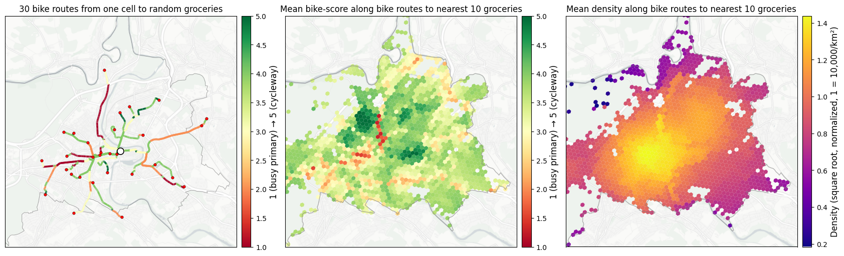
11. Per-edge features aggregated along realised routes¶

Path-first showcase, run BEFORE plugging into the utility computation in §12. In a single routing pass, routing.tiered_path_aggregate returns both the cost ODM and one custom aggregation per registered PathAggregation — letting any per-edge attribute be aggregated along the realised path with no extra Dijkstra calls. The same machinery powers the RouteFeatures in the utility spec (§10): §12 multiplies these aggregations by β_density and β_bike_score to get utility contributions. Here we plot the raw aggregations directly so the building blocks are visible before they’re weighted into utility units.

Two features, both averaged along bike routes from each origin cell to grocery destinations:

``bike_score`` — per-edge quietness (1 busy primary → 5 cycleway / pedestrian path). Tells you whether the typical bike trip from this origin uses pleasant infrastructure or fights traffic.
``density_norm`` — per-edge urban density. Tells you whether the typical bike trip goes through dense centres or quieter periphery.

Per-origin aggregator: nearest-K stores by bike travel time. For each origin, sort destination grocery cells by routed cost ascending, walk through accumulating store counts (the per-cell poi_errands_groceries count), stop when K stores are covered, and take the cost-weighted-quota mean of the per-pair feature across exactly those K stores. “Stores”, not “cells” — a destination cell with multiple groceries contributes proportionally, and the last counted cell may be partially weighted to hit exactly K. Restricted to the cells_to_cells tier.

This replaces an earlier “weighted mean over ALL destinations in the c2c tier” aggregator. The earlier version produced visibly H3-zone-shaped outputs for spatially smooth features (e.g. density_norm), because all cells in one H3 zone shared the entire c2c destination set (the tier is built per-zone-pair for clean mutual exclusion) and a smooth feature’s path-mean over that shared set varies only minimally cell-by-cell. Nearest-K dissolves that artefact: each origin picks its own K nearest stores, so destination sets differ cell-by-cell.

[17]:

bike_pairs = PAIRS["bike"]
costs_odm, feat_aggs = routing.tiered_path_aggregate(
    bike_pairs,
    bike_graph,
    weight="bike_time_s",
    edge_aggregations=[
        routing.PathAggregation("bike_score", edge_bike_score, "mean"),
        routing.PathAggregation("density_norm", "density_norm", "mean"),
    ],
    mask=MASKS["bike"],
    cutoff=60 * 60,
)


def dest_nearest_k_mean_cells_tier(
    feat_odm, costs_odm, pairs, cells_df, value_column, node_column, k: int,
):
    """Per-origin mean of a per-pair feature over the K nearest destinations
    (by routed cost), where "destination unit" is the per-cell count in
    `value_column` (typically a POI count). Restricted to the
    `cells_to_cells` tier.

    For each origin:
      1. Look up destinations + per-pair feature + per-pair cost from c2c.
      2. Filter to destinations with `value_column > 0` (cells holding POIs)
         and finite cost / feature.
      3. Sort ascending by cost.
      4. Walk through, accumulating per-cell counts; stop at K. The last
         counted cell may be partially weighted so the total counts to
         exactly K.
      5. Take the weighted mean of the per-pair feature over those K.

    If fewer than K POIs are reachable from an origin, use what's available
    (no error). Returns a Series keyed by origin snap-node ID."""
    node_to_val = cells_df.groupby(node_column)[value_column].sum().to_dict()
    out = {}
    short_count = 0
    for origin, dest_nodes in pairs.cells_to_cells.items():
        f = feat_odm.cells_to_cells[origin]
        c = costs_odm.cells_to_cells[origin]
        w = np.fromiter(
            (node_to_val.get(d, 0.0) for d in dest_nodes), dtype=float, count=len(dest_nodes)
        )
        valid = np.isfinite(c) & np.isfinite(f) & (w > 0)
        if not valid.any():
            continue
        valid_idx = np.where(valid)[0]
        order = valid_idx[np.argsort(c[valid_idx])]

        used = 0.0
        sum_f = 0.0
        sum_w = 0.0
        for i in order:
            w_i = w[i]
            remaining = k - used
            w_take = w_i if w_i <= remaining else remaining
            sum_f += f[i] * w_take
            sum_w += w_take
            used += w_take
            if used >= k:
                break
        if sum_w > 0:
            out[origin] = sum_f / sum_w
            if used < k:
                short_count += 1
    if short_count:
        print(
            f"  note: {short_count:,} origin(s) had fewer than k={k} reachable "
            f"{value_column!s} units; using whatever was available."
        )
    return pd.Series(out, name=f"mean_along_nearest_{k}_routes")


bike_score_by_node = dest_nearest_k_mean_cells_tier(
    feat_aggs["bike_score"], costs_odm, bike_pairs, cells,
    "poi_errands_groceries", "node_id_bike", k=NEAREST_K_GROCERIES,
)
density_by_node = dest_nearest_k_mean_cells_tier(
    feat_aggs["density_norm"], costs_odm, bike_pairs, cells,
    "poi_errands_groceries", "node_id_bike", k=NEAREST_K_GROCERIES,
)
# Snap-node → cell: multiple cells per node all inherit the same scalar.
bike_score_per_cell = cells["node_id_bike"].map(bike_score_by_node.to_dict())
density_per_cell = cells["node_id_bike"].map(density_by_node.to_dict())
print(
    f"bike_score (1–5) along routes to nearest {NEAREST_K_GROCERIES} groceries: "
    f"median {bike_score_per_cell.median():.2f}, "
    f"P5–P95 [{bike_score_per_cell.quantile(0.05):.2f}, "
    f"{bike_score_per_cell.quantile(0.95):.2f}]"
)
print(
    f"density_norm    along routes to nearest {NEAREST_K_GROCERIES} groceries: "
    f"median {density_per_cell.median():.2f}, "
    f"P5–P95 [{density_per_cell.quantile(0.05):.2f}, "
    f"{density_per_cell.quantile(0.95):.2f}]"
)

  note: 9,609 origin(s) had fewer than k=10 reachable poi_errands_groceries units; using whatever was available.
  note: 9,609 origin(s) had fewer than k=10 reachable poi_errands_groceries units; using whatever was available.
bike_score (1–5) along routes to nearest 10 groceries: median 3.54, P5–P95 [2.29, 4.05]
density_norm    along routes to nearest 10 groceries: median 0.28, P5–P95 [0.11, 0.99]

[18]:

# Pick a representative origin (somewhere in the central city) and K
# RANDOM grocery destinations within the displayed crop box. Random
# sampling — rather than nearest-K — spreads routes across the panel
# so per-edge `bike_score` colouring is actually visible (nearest-K
# would cluster all routes within a few blocks of the origin).
import networkx as nx_for_paths
from shapely.geometry import Point, box  # noqa: E402 — local imports
# `EXAMPLE_ORIGIN_XY` and `EXAMPLE_K_ROUTES` defined at the top of this notebook.

# Origin = the cell whose centroid is nearest to EXAMPLE_ORIGIN_XY.
_origin_pt = Point(*EXAMPLE_ORIGIN_XY)
_origin_cell_id = cells.geometry.centroid.distance(_origin_pt).idxmin()
_origin_node = cells.loc[_origin_cell_id, "node_id_bike"]
_origin_xy = (
    cells.loc[_origin_cell_id].geometry.centroid.x,
    cells.loc[_origin_cell_id].geometry.centroid.y,
)

# Reachability filter — Dijkstra from origin (cutoff matches §3).
_costs_from_origin = nx_for_paths.single_source_dijkstra_path_length(
    bike_graph,
    _origin_node,
    weight="bike_time_s",
    cutoff=15 * 60,
)
# Grocery cells inside the displayed crop AND reachable from the origin.
_crop_box = box(
    CITY_CROP_CENTER_XY[0] - CITY_CROP_HALF_M,
    CITY_CROP_CENTER_XY[1] - CITY_CROP_HALF_M,
    CITY_CROP_CENTER_XY[0] + CITY_CROP_HALF_M,
    CITY_CROP_CENTER_XY[1] + CITY_CROP_HALF_M,
)
_reachable_nodes = set(_costs_from_origin)
_groc_in_crop = cells[
    (cells["poi_errands_groceries"] > 0)
    & cells.geometry.centroid.within(_crop_box)
    & cells["node_id_bike"].isin(_reachable_nodes)
    & (cells["node_id_bike"] != _origin_node)
]
# Random K — deterministic via seeded sampling so the figure is reproducible.
_n = min(EXAMPLE_K_ROUTES, len(_groc_in_crop))
_sampled = _groc_in_crop.sample(n=_n, random_state=42)
_dest_nodes = _sampled["node_id_bike"].tolist()
_dest_xys = [(bike_graph.nodes[n]["x"], bike_graph.nodes[n]["y"]) for n in _dest_nodes]
_paths = [
    nx_for_paths.shortest_path(bike_graph, _origin_node, d, weight="bike_time_s")
    for d in _dest_nodes
]
print(
    f"Example origin: cell {_origin_cell_id} (node {_origin_node}); "
    f"{len(_paths)} random routes to groceries within the crop "
    f"(of {len(_groc_in_crop):,} reachable grocery cells in-crop)."
)

Example origin: cell 8a1f8342cc77fff (node 144881.0); 30 random routes to groceries within the crop (of 129 reachable grocery cells in-crop).

[19]:

# 1×3 — route example (left) | mean bike_score (middle) | mean density (right).
fig, axes = plt.subplots(1, 3, figsize=(21, 6))
figures.plot_routes_on_basemap(
    axes[0],
    bike_graph,
    _paths,
    edge_bike_score,
    cmap="RdYlGn",
    vmin=1,
    vmax=5,
    crop_center_xy=CITY_CROP_CENTER_XY,
    crop_half_m=CITY_CROP_HALF_M,
    origin_xy=_origin_xy,
    dest_xys=_dest_xys,
    city_polygon=CITY_POLYGON,
    crs=cells.crs,
    title=f"{EXAMPLE_K_ROUTES} bike routes from one cell to random groceries",
    label="1 (busy primary) → 5 (cycleway)",
)
figures.plot_city_focus(
    axes[1],
    CITY_POLYGON,
    cells,
    bike_score_per_cell,
    cmap="RdYlGn",
    vmin=1,
    vmax=5,
    crop_center_xy=CITY_CROP_CENTER_XY,
    crop_half_m=CITY_CROP_HALF_M,
    title=f"Mean bike-score along bike routes to nearest {NEAREST_K_GROCERIES} groceries",
    label="1 (busy primary) → 5 (cycleway)",
)
figures.plot_city_focus(
    axes[2],
    CITY_POLYGON,
    cells,
    density_per_cell,
    cmap="plasma",
    crop_center_xy=CITY_CROP_CENTER_XY,
    crop_half_m=CITY_CROP_HALF_M,
    title=f"Mean density along bike routes to nearest {NEAREST_K_GROCERIES} groceries",
    label="Density (square root, normalized, 1 = 10,000/km²)",
)
plt.subplots_adjust(wspace=0.10)
figures.save_figure(fig, "accessibility_path_aggregation")
plt.show()

Saved results/figures_highres/accessibility_path_aggregation.png

../_images/examples_extended_accessibility_31_1.png

12. Per-mode utility ODMs + logsums¶

Pipeline per mode:

Route + per-edge feature aggregations (tiered_path_aggregate): one routing pass yields the node-to-node cost ODM plus the per-pair mean(density_norm) and mean(bike_score) along the realised path.
Lift to geo (reindex_by_geo_unit): cost + features become cell-keyed.
Total cell-to-cell time (overhead.add_geo_overheads): add per-cell origin + destination overheads (in seconds) to the network route time. Result is the realistic door-to-door duration.
Assemble utility (assemble_utility_from_total_time): apply the per-mode β coefficients to total time + route features. Both the linear and log time terms see the same total t_min, so overhead is handled consistently across all utility components (no separate “overhead-as-utility-penalty” step).

Per-mode logsum = ln Σ_j W_j · exp(U_ij), implemented as gravity with a custom decay Decay('exp_u', np.exp) then log of the result. Units are utils; less negative = better access.

[20]:

# `DEST_NEST_SCALE` defined at the top of this notebook.


def make_exp_u_decay(theta: float) -> accessibility.Decay:
    """`Decay` that applies `exp(U / θ)` to per-OD utility values."""
    return accessibility.Decay(
        f"exp_u_theta{theta:.1f}",
        lambda u, _t=theta: np.exp(u / _t),
    )


UTIL_GEO_PAIRS = {}  # label -> TieredODGeoPairs
UTIL_GEO = {}  # label -> TieredODGeoPairs (utility values)
LOGSUM_PER_MODE = {}  # (label, destination) -> per-cell pd.Series (utils)

for label, graph, pairs, mask, time_attr, cutoff_s in ROUTING_PLAN:
    net_label = NETWORK_OF[label]
    node_col = f"node_id_{net_label}"
    ucoef = UTILITY_COEF[label]
    ohcoef = OVERHEAD_COEF[label]

    # 1. Route + per-edge route-feature aggregations (density + bike_score).
    costs, aggs = routing.tiered_path_aggregate(
        pairs,
        graph,
        weight=time_attr,
        edge_aggregations=[
            routing.PathAggregation("density_norm", "density_norm", "mean"),
            routing.PathAggregation("bike_score", edge_bike_score, "mean"),
        ],
        mask=mask,
        cutoff=cutoff_s,
    )
    # 1a. Per-mode floor on route time, BEFORE overhead, across ALL
    #     tiers — eliminates snap-node-coincidence "islands". The
    #     library helper `floor_intrazonal_costs` only touches
    #     cells_to_cells; for the utility logsum we need to floor
    #     cells_to_zones + zones_to_zones too, since those tiers carry
    #     most of the destination weight (and a cell-origin whose snap
    #     node happens to equal a zone's snap node gets a 0-cost route
    #     to that zone's aggregated weight — same artifact as cell-tier
    #     snap-coincidence, just at a different tier).
    costs = floor_all_tiers(costs, min_cost=MIN_ROUTE_S[label])

    # 2. Lift cost + features to geo-keyed form.
    pairs_geo, costs_geo = od_pairs.reindex_by_geo_unit(
        pairs,
        costs,
        cells,
        cell_node_column=node_col,
        zones=zones,
        zone_node_column=node_col,
        **TIER_CUTOFFS[net_label],
    )
    _, density_geo = od_pairs.reindex_by_geo_unit(
        pairs,
        aggs["density_norm"],
        cells,
        cell_node_column=node_col,
        zones=zones,
        zone_node_column=node_col,
        **TIER_CUTOFFS[net_label],
    )
    _, bike_geo = od_pairs.reindex_by_geo_unit(
        pairs,
        aggs["bike_score"],
        cells,
        cell_node_column=node_col,
        zones=zones,
        zone_node_column=node_col,
        **TIER_CUTOFFS[net_label],
    )

    # 3. Add per-cell origin + destination overhead (seconds) → total
    #    cell-to-cell time. Keep `costs_geo` (node-to-node) around for any
    #    downstream consumer; `total_costs_geo` is what utility sees.
    overhead_per_cell_s = overhead.linear_per_cell_overhead(
        cells,
        constant=ohcoef["const"],
        feature_coefficients={
            "density_norm": ohcoef["density"],
            f"snap_dist_{net_label}": ohcoef["snap_dist_s_per_m"],
        },
    )
    total_costs_geo = overhead.add_geo_overheads(
        costs_geo,
        pairs_geo,
        origin_cell=overhead_per_cell_s,
        dest_cell=overhead_per_cell_s,
        cell_to_zone=CELL_TO_ZONE,
    )

    # 4. Assemble utility from total time + route features.
    full_u_geo = assemble_utility_from_total_time(
        total_costs_geo,
        density_geo,
        bike_geo,
        ucoef,
    )
    UTIL_GEO_PAIRS[label] = pairs_geo
    UTIL_GEO[label] = full_u_geo

    # Per-mode logsum per destination. Each destination uses its own
    # nest scale θ — sharp for groceries, broad for employment.
    _, dest_vals = REINDEXED[net_label]
    for d in DESTINATIONS:
        theta = DEST_NEST_SCALE[d]
        decay = make_exp_u_decay(theta)
        grav = accessibility.gravity(
            full_u_geo,
            {d: dest_vals[d]},
            CELL_TO_ZONE,
            [decay],
        )
        with np.errstate(divide="ignore"):
            ls = np.log(grav[(decay.name, d)]) * theta
        # No-destination-reachable origins → log(0) = −∞; surface as NaN
        # so downstream plot bounds aren't dragged to -inf.
        LOGSUM_PER_MODE[(label, d)] = ls.replace([-np.inf, np.inf], np.nan)
        s = LOGSUM_PER_MODE[(label, d)].loc[ORIG_MASK].dropna()
        if len(s):
            print(
                f"  {label:14s} × {d:24s} (θ={theta:.1f}): "
                f"logsum median {s.median():>7.2f}  "
                f"P95 {s.quantile(0.95):>7.2f}"
            )

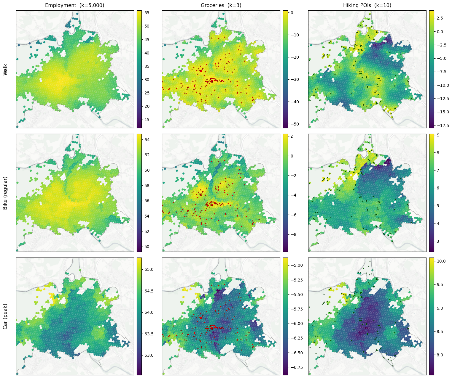
  walk           × employment_total         (θ=6.0): logsum median   24.29  P95   47.68
  walk           × poi_errands_groceries    (θ=1.0): logsum median  -12.42  P95   -2.19
  walk           × poi_leisure_hiking       (θ=3.0): logsum median   -5.01  P95    0.54
  bike_regular   × employment_total         (θ=6.0): logsum median   48.37  P95   62.18
  bike_regular   × poi_errands_groceries    (θ=1.0): logsum median   -2.40  P95    0.17
  bike_regular   × poi_leisure_hiking       (θ=3.0): logsum median    5.47  P95    7.81
  car_peak       × employment_total         (θ=6.0): logsum median   62.91  P95   64.45
  car_peak       × poi_errands_groceries    (θ=1.0): logsum median   -5.77  P95   -5.17
  car_peak       × poi_leisure_hiking       (θ=3.0): logsum median    8.80  P95   10.07

Per-mode logsum maps (3 modes × 3 destinations), same city-shaped clip as §9.

[21]:

fig, axes = plt.subplots(3, 3, figsize=(18.5, 16))
for row, (label, _, _, _, _, _) in enumerate(ROUTING_PLAN):
    for col, d in enumerate(DESTINATIONS):
        figures.plot_city_focus(
            axes[row, col],
            CITY_POLYGON,
            cells,
            LOGSUM_PER_MODE[(label, d)],
            pois=pois_overlay_for(d),
            crop_center_xy=CITY_CROP_CENTER_XY,
            crop_half_m=CITY_CROP_HALF_M,
            title="",
        )
        if row == 0:
            axes[row, col].set_title(DEST_LABELS[d], pad=8)
plt.subplots_adjust(wspace=0.10, hspace=0.05)
for row, (label, _, _, _, _, _) in enumerate(ROUTING_PLAN):
    pos = axes[row, 0].get_position()
    fig.text(
        pos.x0 - 0.012,
        (pos.y0 + pos.y1) / 2,
        MODE_LABELS[label],
        rotation=90,
        va="center",
        ha="center",
        fontsize=figures.LABEL_SIZE,
    )
figures.save_figure(fig, "accessibility_per_mode_logsum")
plt.show()

Saved results/figures_highres/accessibility_per_mode_logsum.png

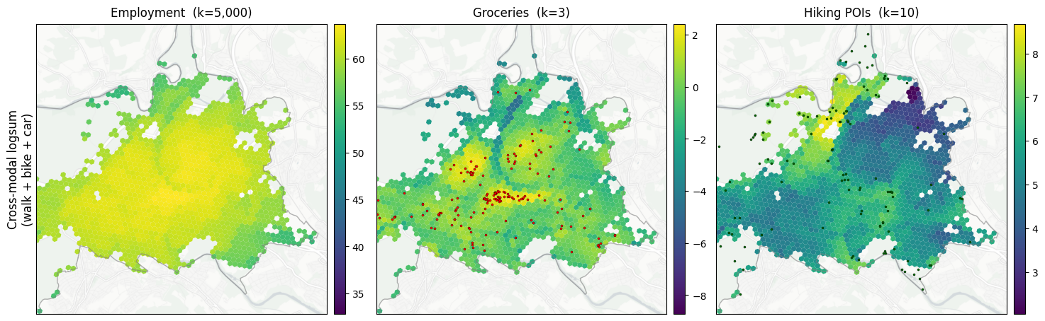
../_images/examples_extended_accessibility_35_1.png

13. Cross-modal logsum¶

Combine the three per-mode utility ODMs via a utility-domain logsum aggregator (ln Σ_m exp(U_ijm) per OD pair), then apply gravity + log to get the cross-modal accessibility:

A_i = ln Σ_j W_j · Σ_m exp(U_ijm)

The per-mode logsums above tell you how reachable destinations are by each mode separately; the cross-modal logsum tells you how reachable they are if the agent picks whichever mode gives the highest utility per trip. This is the multi-modal half of the multi-scale × multi-modal combination that the toolkit paper centres on.

[22]:

def logsum_utility(stacked: np.ndarray) -> np.ndarray:
    """Cross-modal logsum in utility space: ln Σ_m exp(U_m) per OD pair.

    NaN entries (mode-unreachable for that OD pair) contribute 0 to the sum.
    """
    exp_terms = np.exp(stacked)
    exp_terms = np.where(np.isnan(exp_terms), 0.0, exp_terms)
    sum_exp = exp_terms.sum(axis=0)
    with np.errstate(divide="ignore"):
        return np.log(sum_exp)


combined_pairs, combined_u = od_pairs.aggregate_across_modes(
    {label: (UTIL_GEO_PAIRS[label], UTIL_GEO[label]) for label, _, _, _, _, _ in ROUTING_PLAN},
    aggregator=logsum_utility,
)
combined_dest_vals = {
    d: od_pairs.dest_values_geo(d, combined_pairs, cells, zones=zones) for d in DESTINATIONS
}
# Per-destination nest scale on the destination logsum — same θ as in
# §12 so the per-mode and cross-modal results are on the same scale.
CROSS_LOGSUM = {}
for d in DESTINATIONS:
    theta = DEST_NEST_SCALE[d]
    decay = make_exp_u_decay(theta)
    grav = accessibility.gravity(
        combined_u,
        {d: combined_dest_vals[d]},
        CELL_TO_ZONE,
        [decay],
    )
    with np.errstate(divide="ignore"):
        ls = np.log(grav[(decay.name, d)]) * theta
    CROSS_LOGSUM[d] = ls.replace([-np.inf, np.inf], np.nan)

fig, axes = plt.subplots(1, 3, figsize=(18, 6))
for col, d in enumerate(DESTINATIONS):
    figures.plot_city_focus(
        axes[col],
        CITY_POLYGON,
        cells,
        CROSS_LOGSUM[d],
        pois=pois_overlay_for(d),
        crop_center_xy=CITY_CROP_CENTER_XY,
        crop_half_m=CITY_CROP_HALF_M,
        title="",
    )
    axes[col].set_title(DEST_LABELS[d], pad=8)
plt.subplots_adjust(wspace=0.10)
pos = axes[0].get_position()
fig.text(
    pos.x0 - 0.012,
    (pos.y0 + pos.y1) / 2,
    "Cross-modal logsum\n(walk + bike + car)",
    rotation=90,
    va="center",
    ha="center",
    fontsize=figures.LABEL_SIZE,
)
figures.save_figure(fig, "accessibility_cross_modal_logsum")
plt.show()

Saved results/figures_highres/accessibility_cross_modal_logsum.png

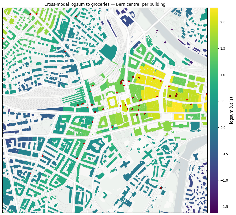
../_images/examples_extended_accessibility_37_1.png

14. Neighborhood zoom — accessibility per building¶

Cells are H3 res 10 (~130 m), so each cell aggregates a handful of buildings. Joining the per-cell logsum back to the underlying building layer (via prepare/’s building_to_cell mapping) lets us colour every building by its cell’s cross-modal accessibility — the same numbers as §13 above, projected onto the unit of analysis that downstream consumers usually care about.

Below: a ~1.4 × 1.4 km window over central Bern, every building coloured by its cell’s cross-modal logsum to groceries, with the car-network edges (white) and supermarket POIs (red) on top.

[23]:

buildings = gpd.read_file(PREPARED_DIR / "buildings.gpkg")
b2c = pd.read_csv(PREPARED_DIR / "building_to_cell.csv", index_col=0)
# buildings.gpkg and building_to_cell.csv are row-aligned (one row per
# building, in the same order they were emitted in prep).
buildings["cell_id"] = b2c["cell_id"].values
buildings["logsum_groceries"] = buildings["cell_id"].map(CROSS_LOGSUM["poi_errands_groceries"])

fig, ax = plt.subplots(figsize=(10, 10))
figures.plot_neighborhood_zoom(
    ax,
    buildings,
    center_xy=NEIGHBORHOOD_CENTER_XY,
    half_m=NEIGHBORHOOD_HALF_M,
    values=buildings["logsum_groceries"],
    network=car_graph,
    title=f"Cross-modal logsum to groceries — {LOCATION_LABEL} centre, per building",
    label="logsum (utils)",
)
# POI overlay on top of buildings + network — supermarkets visible
# within the crop window only.
sm = pois[pois["poi_errands_groceries"] > 0]
ax.scatter(
    sm.geometry.x, sm.geometry.y, s=22, color="red", edgecolor="black", linewidth=0.5, zorder=6
)
plt.tight_layout()
figures.save_figure(fig, "accessibility_neighborhood_buildings")
plt.show()

Saved results/figures_highres/accessibility_neighborhood_buildings.png

../_images/examples_extended_accessibility_39_1.png

What this notebook does NOT do¶

Tutorial-scope analysis using published-paper edge-weight coefficients (Miotti et al., Transportation, 20XX) and approximate per-mode utility coefficients informed by an ongoing project. It deliberately omits things production code would do:

One variant per mode. Walk + regular bike + car peak. The paper has more (e-bike 25/45, car off-peak/night) — see `projects/lumos/ <https://github.com/mmiotti/aperta-lab/tree/main/src/projects/lumos>`__ for the full variant matrix with peak vs off-peak congestion deltas and bike vs e-bike comparisons.
Cell-tier overheads only. Production aggregates destination overhead at middle / far tiers via centroid-to-centroid distance. Cells are small enough here that the difference is minor.
No ``overhead_*_dist`` term. The published coefficient table doesn’t have it; production may add it back per regional fit.
Edge weights are paper-derived, not re-calibrated for this region. To re-derive them from ground-truth travel times, see calibrate_edge_weights.ipynb; to add a traffic-flow / congestion feature, see traffic_flows.ipynb. Neither is wired into this notebook by design — each showcase notebook stands alone.