`flow_estimate` — per-edge AADT as a congestion proxy¶

⚠️ Data availability. This notebook requires two ground-truth inputs that aperta cannot redistribute under their source terms: Swiss ASTRA traffic-counter readings (data/ground_truth/ traffic_counters.gpkg) and Google-Maps-derived car travel times (data/ground_truth/travel_times_car_peak.csv, the same file used by calibrate_edge_weights.ipynb). The notebook is shipped as documentation of the flow-estimation method and the counter-fit diagnostics — the model spec, sampling logic, and evaluation are inspectable end-to-end — but cells that read the ground-truth files will not run without them. The rest of the extended example (prepare/, accessibility.ipynb) runs entirely on public OSM data. A public-data version is planned for a future release.

Estimates per-edge AADT for the car network via cost-decay-weighted nested-betweenness sampling. The output is a rough proxy for “traffic pressure” on each edge, suitable as a feature in car edge-weight calibration (e.g. a BPR-style (V/C)² congestion multiplier feeding into typical-time-of-day speeds for accessibility). It is NOT a traffic assignment.

Two simplifications worth flagging upfront. No stochastic routing — every OD pair takes a single deterministic shortest path, so flow piles up on the “winner” route and any parallel alternative sees nothing. No capacity-based slowdown — a saturated motorway and an empty one carry the same edge weight, so loading keeps stacking on the highest-rank corridor even past capacity. The net effect is over-prediction on highways / main roads and under-prediction on parallel local roads. That’s acceptable for a relative pressure feature feeding edge-speed calibration; it’s not acceptable for road design. The library calibration loop (see aperta-lab/projects/lumos/) fits BPR multipliers against observed counters to compensate on the way to typical edge speeds.

Cost-distribution target. Each origin’s sampled trip costs are reweighted to match a target P(C) read directly from the ground-truth Google-Maps trip times — equal-probability percentile bins over [MIN_COST_S, MAX_COST_S]. This corrects the sparse-periphery bias of plain cost-weighted destination sampling, where each periphery origin would otherwise carry too much weight on its few in-range neighbours. bin_adjusted_dest_weights does the reweighting; nested_node_sample then draws destinations proportional to the adjusted weights with no separate cost-decay factor.

Tunable knobs (priors here, fitted in production):

N_BINS — granularity of the percentile-binned target P(C).
MIN_COST_S, MAX_COST_S — survey-trim window. Trips outside it are excluded from the target; destinations whose realised cost falls outside get zero sampling weight, so OD pairs beyond MAX_COST_S (or implausibly below MIN_COST_S) don’t contribute.
TRIPS_PER_PERSON_PER_DAY — overall scaling to vehicles/day, constant prior of 1.5.

Design choices¶

Nested cell + zone hierarchy. Origins and short-trip destinations use H3-res-10 cells (~130 m); medium- and far-tier destinations aggregate to H3-res-8 zones (~460 m). Cell-level origins matter because intra-zone short trips contribute disproportionately to local-road flows — collapsing them to zone-only sampling systematically under-counts low-volume residential edges.

Origins NOT restricted to AOI. Trips originating outside the AOI but passing through it contribute to observed counter readings, so restricting origins to AOI would systematically under-predict near the boundary.

[1]:

import warnings
from pathlib import Path

import geopandas as gpd
import matplotlib.pyplot as plt
import numpy as np
import pandas as pd

from aperta import (
    calibration,
    network_processing,
    od_pairs,
    routing,
    traffic_flows,
)
from aperta.network_processing import OSM_HIGHWAY_RANKS

warnings.filterwarnings('ignore', category=FutureWarning)
warnings.filterwarnings('ignore', category=UserWarning, module='geopandas')

Parameters¶

Everything tunable in one place.

[2]:

PREPARED_DIR = Path('data/prepared')
GROUND_TRUTH_DIR = Path('data/ground_truth')
LOCATION_LABEL = 'Bern'   # for plot titles; keep in sync with prepare/1_download

# Counter-to-edge snap. Highway counters get a wider radius (sparser
# layout, lower risk of catching a parallel local road) but can only
# snap to highway edges. Bearing tolerance prevents opposite-direction
# counters from cross-snapping on two-way roads.
HIGHWAY_RADIUS_M = 25.0
NON_HIGHWAY_RADIUS_M = 10.0
BEARING_TOL_DEG = 20.0

# Initial per-edge durations: base = length / speed_kph, with
# multiplicative + additive corrections for density and intersection /
# signal load. Features from `prepare/5_density`; coefficients are
# off-peak car priors.
INITIAL_MULT = {'density_norm': 0.25}
INITIAL_ADD = {'is_4way': 3.0, 'is_traffic_signal': 7.0}

# OD-tier radii (CRS metres) + travel-time cutoff.
R_CELLS_M = 1_500
R_MEDIUM_M = 10_000
R_ZONES_M = 100_000
# Cutoff at 30 min: since they area does not systematically allow for longer trips than
# that, results become biased if the cutoff is set higher.
CAR_TIME_CUTOFF_S = 1800

# Inner-core polygon for counter filtering (AOI shrunk by this buffer)
# to avoid boundary effects on the evaluation set.
INNER_BUFFER_M = 15_000.0

# Sampling. Origins drawn population-weighted (with replacement, then
# deduped); destinations drawn per-origin proportional to the
# bin-adjusted weights (§3).
N_ORIG = 10_000
N_DEST = 10
RNG_SEED = 42

# Cost-distribution target P(C). `N_BINS` is the granularity of the
# percentile-binned target (20 ≙ 5%-bins). `MIN_COST_S` / `MAX_COST_S`
# trim the survey to a plausible trip-time window — they become the 0th
# and 100th percentiles of the target distribution, so destinations
# with realised cost below `MIN_COST_S` or above `MAX_COST_S` get zero
# sampling weight and are excluded from the flow estimate.
N_BINS = 20
MIN_COST_S = 0.0
MAX_COST_S = 7200.0   # 2 h — well above the survey's 99th percentile

# Volume scaling — vehicles per person per day. Reasonable prior;
# production calibration fits this against observed counters.
TRIPS_PER_PERSON_PER_DAY = 1.8

1. Load inputs¶

Graph + cells + zones + counters. The counters file holds directional point counters with traffic_cars, bearing_deg, and per-tier flags (is_highway, is_main, is_local).

[3]:

car_graph = network_processing.load_consolidated_graphml(
    PREPARED_DIR / 'car_graph.graphml')
print(f"Car graph: {car_graph.number_of_nodes():,} nodes / "
      f"{car_graph.number_of_edges():,} edges")

zones = gpd.read_file(PREPARED_DIR / 'zones.gpkg').set_index('zone_id')
zones['pop_plus_emp'] = zones['population'] + zones['employment_total']
zones = zones.rename(columns={'node_id_car': 'node_id'})
total_pop = float(zones['population'].sum())
print(f"Zones: {len(zones):,} (Σ pop {total_pop:,.0f})")

cells = gpd.read_file(PREPARED_DIR / 'cells.gpkg').set_index('cell_id')
cells['pop_plus_emp'] = cells['population'] + cells['employment_total']
# Drop POI-only cells (no orig weight + no dest weight = pure routing cost).
cells = cells[cells['pop_plus_emp'] > 0].copy()
cells = cells.rename(columns={'node_id_car': 'node_id'})
print(f"Cells: {len(cells):,} (after dropping pop+emp=0)")

counters_all = gpd.read_file(GROUND_TRUTH_DIR / 'traffic_counters.gpkg')
print(f"Counters: {len(counters_all):,} "
      f"(highway: {int(counters_all['is_highway'].sum()):,}, "
      f"main: {int(counters_all['is_main'].sum()):,}, "
      f"local: {int(counters_all['is_local'].sum()):,})")

# Restrict the evaluation set to counters in the AOI core (AOI shrunk
# by INNER_BUFFER_M): counters near the edge see traffic going to /
# from places outside the model area that the simulation can't
# generate. Inner-core counters avoid that edge-effect bias.
dest_polygon = gpd.read_file(PREPARED_DIR / 'dest_polygon.gpkg').geometry.iloc[0]
inner_polygon = dest_polygon.buffer(-INNER_BUFFER_M)
in_inner = counters_all.geometry.within(inner_polygon)
counters = counters_all[in_inner].copy()
print(f"  inside core (dest_polygon − {INNER_BUFFER_M / 1000:.0f} km): "
      f"{len(counters):,} — used for evaluation below")

legs = pd.read_csv(GROUND_TRUTH_DIR / 'travel_times_car_peak.csv')

Car graph: 33,860 nodes / 90,839 edges
Zones: 8,903 (Σ pop 1,551,024)
Cells: 139,837 (after dropping pop+emp=0)
Counters: 4,691 (highway: 447, main: 3,849, local: 395)
  inside core (dest_polygon − 15 km): 807 — used for evaluation below

2. Snap counters to the car-graph edges¶

Per-counter eligibility restricts the search to edges of the matching road tier so a highway counter can’t snap to a parallel residential road. Each matched counter is tagged with the OSM highway_rank (-1 = service/unclassified … 7 = motorway) — useful downstream for filtering e.g. counters['highway_rank'] >= 3.

[4]:

def _edge_rank_and_tier(d) -> tuple[int, str]:
    """Return (OSM rank, tier bucket) for an edge attribute dict."""
    hwy = d.get('highway')
    if isinstance(hwy, list):
        hwy = hwy[0] if hwy else None
    rank = OSM_HIGHWAY_RANKS.get(hwy, -1)
    if rank >= 6: tier = 'highway'    # motorway / trunk
    elif rank >= 3: tier = 'main'     # primary / secondary / tertiary
    else: tier = 'local'              # residential / service / unknown
    return rank, tier

for _, _, _, d in car_graph.edges(keys=True, data=True):
    d['_highway_rank'], d['_tier'] = _edge_rank_and_tier(d)

search_radius = counters['is_highway'].map(
    {1: HIGHWAY_RADIUS_M, 0: NON_HIGHWAY_RADIUS_M})

def _eligible_for_counter(counter_row, candidate_edges):
    if counter_row['is_highway']:    wanted = 'highway'
    elif counter_row['is_main']:     wanted = 'main'
    else:                            wanted = 'local'
    return candidate_edges[candidate_edges['_tier'] == wanted]

snapped = calibration.snap_counters_to_edges(
    counters, car_graph,
    search_radius=search_radius,
    bearing_tol_deg=BEARING_TOL_DEG,
    eligible_edges=_eligible_for_counter,
)
counters = counters.join(snapped)
counters['highway_rank'] = [
    car_graph[u][v][k]['_highway_rank'] if pd.notna(u) else np.nan
    for u, v, k in zip(counters['u'], counters['v'], counters['k'])
]
n_matched = counters['u'].notna().sum()
print(f"Snapped: {n_matched:,} of {len(counters):,} counters "
      f"({n_matched / len(counters) * 100:.1f}%)")
for tier_col, label in [('is_highway', 'highway'), ('is_main', 'main'),
                        ('is_local', 'local')]:
    mask = counters[tier_col] == 1
    n_tot = int(mask.sum())
    n_ma = int((mask & counters['u'].notna()).sum())
    if n_tot:
        print(f"  {label:8s}: {n_ma:,} of {n_tot:,} "
              f"({n_ma / n_tot * 100:.1f}%)")
_rank_counts = (counters.loc[counters['u'].notna(), 'highway_rank']
                .astype(int).value_counts().sort_index())
print(f"  matched edges by OSM highway rank: {_rank_counts.to_dict()}")

Snapped: 676 of 807 counters (83.8%)
  highway : 53 of 53 (100.0%)
  main    : 606 of 684 (88.6%)
  local   : 17 of 70 (24.3%)
  matched edges by OSM highway rank: {-1: 3, 2: 14, 3: 105, 4: 266, 5: 235, 6: 2, 7: 51}

3. Build the routing inputs¶

Per-edge initial durations, OD pairs across the three tiers, costs along each pair, sampling weights, and the survey-derived cost-distribution target used to bin-adjust those weights.

[5]:

# Per-edge initial durations.
KMH_TO_MS = 1.0 / 3.6
for u, v, k, d in car_graph.edges(keys=True, data=True):
    base = float(d['length']) / (float(d['speed_kph']) * KMH_TO_MS)
    mult_term = base * sum(c * float(d[f]) for f, c in INITIAL_MULT.items())
    add_term = sum(c * float(d[f]) for f, c in INITIAL_ADD.items())
    d['duration_initial'] = max(base + mult_term + add_term, base * 0.2)

# Tiered OD pairs + per-pair routing costs.
cells['_dest_weight'] = cells['employment_total']
zones['_dest_weight'] = zones['employment_total']
pairs = od_pairs.get_pairs(
    cells, r_cells=R_CELLS_M, node_column='node_id',
    zones=zones, r_zones=R_ZONES_M, r_medium=R_MEDIUM_M,
)
costs = routing.tiered_path_costs(
    pairs, car_graph, weight='duration_initial', cutoff=CAR_TIME_CUTOFF_S,
)
orig_weights = od_pairs.node_values(
    'pop_plus_emp', cells, 'node_id',
    list(pairs.cells_to_cells.keys()))
dest_weights = od_pairs.dest_values(
    '_dest_weight', pairs, cells, 'node_id', zones=zones)
cell_to_zone_node = od_pairs.build_cell_to_zone_node_map(
    cells, zones, node_column='node_id')

# Cost-distribution target P(C). Survey trip times are trimmed to
# [MIN_COST_S, MAX_COST_S]; equal-probability percentile bins over the
# in-range subset become the target each origin is rescaled to match.
# The endpoint percentiles are then forced to (MIN_COST_S, MAX_COST_S)
# so the helper's in-range mask matches the user's clip window exactly.
_survey_costs = legs.loc[
    (legs['time_measured'] >= MIN_COST_S)
    & (legs['time_measured'] <= MAX_COST_S),
    'time_measured',
].to_numpy()
bin_edges = traffic_flows.percentile_bin_edges(_survey_costs, n_bins=N_BINS)
bin_edges[0] = MIN_COST_S
bin_edges[-1] = MAX_COST_S
print(f"Cost-bin edges ({N_BINS} bins, clipped to "
      f"[{MIN_COST_S:.0f}, {MAX_COST_S:.0f}] s; "
      f"n_survey={len(_survey_costs):,}):")
print(f"  {[f'{e:.0f}' for e in bin_edges]}")

adjusted_dest_weights = traffic_flows.bin_adjusted_dest_weights(
    pairs, costs, dest_weights, bin_edges,
)

Cost-bin edges (20 bins, clipped to [0, 7200] s; n_survey=49,347):
  ['0', '137', '191', '239', '288', '339', '392', '452', '515', '585', '664', '751', '848', '960', '1093', '1257', '1469', '1748', '2172', '3030', '7200']

4. Run the flow estimation¶

Sample population-weighted origins; for each origin sample destinations proportional to the bin-adjusted weights from §3; accumulate shortest-path betweenness; scale counts to AADT.

AADT scaling. nested_node_sample dedupes the with-replacement origin draw, so the actual sample count is len(nested_sample) · N_DEST (not the nominal N_ORIG · N_DEST). Scaling by the actual count keeps results invariant to the N_ORIG / N_DEST split.

Cost-distribution correction. Sampling weights are pre-adjusted per origin per percentile bin in §3 so the realised trip-cost distribution from each origin matches the survey-derived target P(C). Replaces the lognormal cost-decay prior used in earlier versions, which under-normalised sparse-periphery origins and inflated through-corridor flows as the analysis area grew. With the correction in place, cost_to_weight becomes the identity (the cost-dependence is already baked into adjusted_dest_weights).

[6]:

rng = np.random.RandomState(RNG_SEED)
nested_sample = traffic_flows.nested_node_sample(
    pairs=pairs, weights=adjusted_dest_weights, costs=costs,
    cell_to_zone_node=cell_to_zone_node, orig_weights=orig_weights,
    cost_to_weight=np.ones_like, n_orig=N_ORIG, n_dest=N_DEST,
    random_state=rng,
)
edge_bc = network_processing.get_nested_edge_betweenness(
    car_graph, nested_sample, weight='duration_initial',
    cutoff=od_pairs.max_cost(costs),  # correctness-preserving Dijkstra cap
)
aadt_scale = (total_pop * TRIPS_PER_PERSON_PER_DAY) / (len(nested_sample) * N_DEST)
flows = edge_bc * aadt_scale
network_processing.set_nx_edge_attributes_filled(
    car_graph, flows.to_dict(), 'flow_estimate', fill_value=0.0)
print(f"flows (veh/day): "
      f"median {flows.median():.0f}, "
      f"P95 {flows.quantile(0.95):.0f}, "
      f"max {flows.max():.0f}")

OUTPUT_PATH = PREPARED_DIR / 'flow_estimate.csv'
flows_df = pd.DataFrame(
    [(u, v, k, float(flows.get((u, v, k), 0.0)))
     for u, v, k in car_graph.edges(keys=True)],
    columns=['u', 'v', 'k', 'flow_estimate'],
)
flows_df.to_csv(OUTPUT_PATH, index=False)
print(f"Saved {len(flows_df):,} rows to {OUTPUT_PATH}")

flows (veh/day): median 476, P95 5002, max 47920
Saved 90,839 rows to data/prepared/flow_estimate.csv

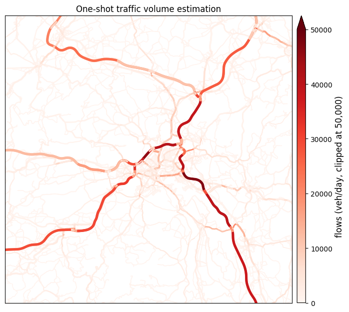
5. Diagnostics¶

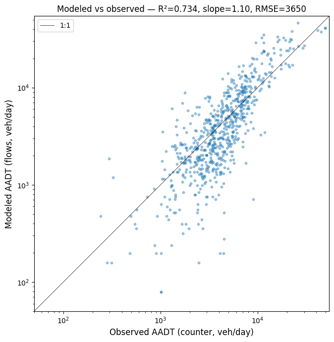
Scatter of modeled vs observed AADT at matched counters (the fit this rough proxy achieves at the prior parameters), and a per-edge flow map for visual sanity-checking. The over-/under-prediction pattern flagged in the header is visible on both: highway points typically sit above the 1:1 line, local-road points below.

[7]:

ev = calibration.evaluate_against_counters(flows, counters)
print(f"Fit at counters: R²={ev['r2']:.3f}, slope={ev['slope']:.3f}, "
      f"RMSE={ev['rmse']:.0f}, n={ev['n_matched']:,}")

import _figures as figures   # noqa: E402  — project-local plot helpers
m = ev['merged']
fig, ax = plt.subplots(figsize=(7, 7))
ax.scatter(m['observed'], m['modeled'], s=10, alpha=0.4, color='tab:blue')
lim = float(max(m['observed'].max(), m['modeled'].max())) * 1.1
ax.plot([1, lim], [1, lim], color='black', linewidth=0.5, label='1:1')
ax.set_xscale('log'); ax.set_yscale('log')
ax.set_xlim(50, lim); ax.set_ylim(50, lim)
ax.set_xlabel('Observed AADT (counter, veh/day)')
ax.set_ylabel('Modeled AADT (flows, veh/day)')
ax.set_title(f'Modeled vs observed — R²={ev["r2"]:.3f}, '
             f'slope={ev["slope"]:.2f}, RMSE={ev["rmse"]:.0f}')
ax.set_aspect('equal'); ax.legend()
plt.tight_layout()
figures.save_figure(fig, 'flow_baseline_evaluation_scatter', ext='pdf')
plt.show()

Fit at counters: R²=0.734, slope=1.105, RMSE=3650, n=671
Saved results/figures_highres/flow_baseline_evaluation_scatter.pdf

../_images/examples_extended_traffic_flows_13_1.png

[8]:

stress_arr = np.array([float(d.get('flow_estimate', 0.0))
                       for _, _, d in car_graph.edges(data=True)])

# Standardised paper-figure crop: 20 × 20 km square centred on Bern
# (same centre as the accessibility figures so the four paper figures
# show the same area at the same scale).
PAPER_CROP_CENTER_XY = (2_599_000, 1_200_500)
PAPER_CROP_HALF_M    = 15_000
xlim = (PAPER_CROP_CENTER_XY[0] - PAPER_CROP_HALF_M,
        PAPER_CROP_CENTER_XY[0] + PAPER_CROP_HALF_M)
ylim = (PAPER_CROP_CENTER_XY[1] - PAPER_CROP_HALF_M,
        PAPER_CROP_CENTER_XY[1] + PAPER_CROP_HALF_M)

FLOW_VMAX = 50_000   # AADT cap for the colour scale

fig, ax = plt.subplots(figsize=(7, 6.5))
figures.plot_network_map(
    ax, car_graph, flows,
    cbar_label=f'flows (veh/day, clipped at {FLOW_VMAX:,})',
    title=('One-shot traffic volume estimation'),
    xlim=xlim, ylim=ylim,
    vmax=FLOW_VMAX,
)
# ax.plot(*inner_polygon.exterior.xy,
#         color='black', linewidth=1.0, linestyle='--',
#         label='inner polygon (calibration region)', zorder=5)
# ax.scatter(counters_all.geometry.x, counters_all.geometry.y,
#            s=18, facecolor='white', edgecolor='black', linewidth=0.6,
#            label=f'counters', zorder=6)
# _legend = ax.legend(loc='upper right', framealpha=0.9, fontsize=9)
# _legend.set_zorder(20)   # above the counter dots
plt.tight_layout()
figures.save_figure(fig, 'flow_estimate_map')
plt.show()

Saved results/figures_highres/flow_estimate_map.png

../_images/examples_extended_traffic_flows_14_1.png

What this notebook does NOT do¶

Beyond the no-stochastic-routing / no-capacity simplifications flagged in the header:

No automated calibration against counters. With the cost distribution now anchored by survey data, the only free knob is TRIPS_PER_PERSON_PER_DAY (a 1.5 prior here). Production coordinate-descents it against counters with a slope-vs-RMSE trade-off and an inner-vs-outer counter filter.
Output isn’t consumed by ``accessibility.ipynb``. Each showcase notebook stands alone. Production does feed flow_estimate into edge-weight calibration as a (V/C)² BPR-style multiplicative feature — that’s the link from this notebook’s output to typical edge speeds.
No capacity-normalised stress map. Dividing flows by lanes × per-lane capacity and raising to β (≈ 2 or 4, BPR convention) highlights bottlenecks regardless of road class, but is a deep dive. See aperta-lab/projects/lumos/.

flow_estimate — per-edge AADT as a congestion proxy¶