Calibrate car edge weights against observed trip times

⚠️ Data availability. This notebook requires ground-truth car travel times derived from the Google Maps Directions API on origin coordinates from the protected Swiss MTMC mobility survey (data/ground_truth/travel_times_car_peak.csv). Aperta cannot redistribute this file under its source terms. The notebook is shipped as documentation of the calibration method — the model spec, fitting loop, diagnostics, and outputs are inspectable end-to-end — but cells past §4 will not run without the private inputs. The rest of the extended example (prepare/, accessibility.ipynb) runs entirely on public OSM data. A public-data version of this notebook is planned for a future release; any replacement data with the same schema (orig_x, orig_y, dest_x, dest_y, time_measured, dist_measured, dist_line) drops in directly.

Iteratively calibrates the per-edge duration formula for cars against Google-Maps-derived point-to-point travel times. All inputs come from prepare/: the consolidated car graph (prepare/1_download for topology + intersection / signal flags + OSM speeds) and per-edge density_norm (prepare/5_density).

Calibration model (see aperta.calibration module docstring):

trip_time = α · baseline_time
          + Σ_m coef_m · (baseline_time · m_avg_along_path)
          + Σ_a coef_a · (a_sum_along_path)
          + Σ_e coef_e · (e_at_origin + e_at_destination)
          + constant

baseline_time is per-edge length / speed_kph (with speed_kph from OSM maxspeed + per-highway fallback, set in prepare/1_download). This stays unchanged across iterations — the calibration learns the multiplicative correction α and the per-feature coefficients.

Ground truth: Google-Maps car_pessimistic.csv (~50 k legs), columns orig_x, orig_y, dest_x, dest_y, time_measured, dist_measured, dist_line. Origin coordinates are derived from the protected MTMC survey, so this specific data file isn’t public — the workflow itself is the reusable part. Replacement data with the same schema would slot in directly.

import warnings
from pathlib import Path

import geopandas as gpd
import matplotlib.pyplot as plt
import networkx as nx
import numpy as np
import osmnx as ox
import pandas as pd
from shapely.geometry import Point

from aperta import calibration, geo_processing, network_processing, routing_prep

warnings.filterwarnings('ignore', category=FutureWarning)
warnings.filterwarnings('ignore', category=UserWarning, module='geopandas')

PREPARED_DIR = Path('data/prepared')
GROUND_TRUTH_PATH = Path('data/ground_truth/travel_times_car_peak.csv')
CRS_METRIC = 'EPSG:2056'

1. Load graph + cells + ground truth

car_graph = network_processing.load_consolidated_graphml(
    PREPARED_DIR / 'car_graph.graphml')
print(f"Car graph: {car_graph.number_of_nodes():,} nodes / "
      f"{car_graph.number_of_edges():,} edges")

# Mode-aware preparation: keeps the graph directed (car defaults), precomputes
# the largest strongly connected component as the snap-eligible node set.
# Passing `eligible_node_ids=car_prepared.snap_eligible_nodes` to the
# calibration below prevents trip endpoints from snapping to trapped nodes
# (which would otherwise produce spurious routing failures and contaminate
# the OLS fit).
car_prepared = routing_prep.prepare_network(car_graph, 'car')
car_graph = car_prepared.graph
print(f"  Snap-eligible (largest SCC): {len(car_prepared.snap_eligible_nodes):,} nodes "
      f"({100 * len(car_prepared.snap_eligible_nodes) / car_graph.number_of_nodes():.1f}%)")

cells = gpd.read_file(PREPARED_DIR / 'cells.gpkg').set_index('cell_id')
cells['pop_plus_emp'] = cells['population'] + cells['employment_total']
print(f"Cells: {len(cells):,}")

legs = pd.read_csv(GROUND_TRUTH_PATH)
print(f"Ground-truth legs: {len(legs):,} "
      f"(median time {legs['time_measured'].median():.0f} s, "
      f"median dist {legs['dist_measured'].median():.0f} m)")

Car graph: 33,860 nodes / 90,839 edges
  Snap-eligible (largest SCC): 33,837 nodes (99.9%)
Cells: 142,209
Ground-truth legs: 49,773 (median time 671 s, median dist 5685 m)

2. Per-edge features (from prep)

All features used by the calibration formula below are already on the graph from the prep notebooks:

• speed_kph per edge (from prepare/1_download)

• density_norm, is_4way, is_traffic_signal per edge (from prepare/5_density)

These attrs are cast back to floats on graphml load via network_processing.CONSOLIDATED_EDGE_DTYPES, which load_consolidated_graphml applies. Just a diagnostic.

speeds = np.array([float(d['speed_kph'])
                   for _, _, d in car_graph.edges(data=True)])
print(f"Baseline car edge speeds: median {np.median(speeds):.0f} km/h, "
      f"range {speeds.min():.0f}–{speeds.max():.0f} km/h.")

Baseline car edge speeds: median 30 km/h, range 10–120 km/h.

3. Calibrate

Three feature classes enter the OLS fit:

• multiplier: scales baseline duration. coef · baseline ·   feature_value. Density would belong here — left empty in this showcase to keep the model interpretable.

• additive_route: adds seconds per occurrence, summed along the routed path. Intersection counts, traffic signals.

• additive_endpoint: adds seconds based on the value of a node attribute at origin and destination. Snap distance (cell centroid → nearest network node).

Initial coefficients chosen close to typical car off-peak values so the first iteration starts near a plausible regime. n_iterations=3 is usually enough to converge.

result = calibration.calibrate_edge_weights(
    car_graph, legs,
    baseline_speed_attr='speed_kph',
    multiplier_features={
        'density_norm':      0.2,    # Higher density = lower speeds
    },
    additive_route_features={
        # is_t_junction dropped — multicollinear with density.
        'is_4way':           2.6,    # secs per 4-way intersection
        'is_traffic_signal': 4.4,    # secs per signalised intersection
    },
    additive_endpoint_features={
        # Density at orig/dest dropped — overfitting risk on small n.
        'snap_dist':         0.2,    # secs per metre of first-mile distance
    },
    constant=True,
    n_iterations=3,
    min_trip_distance=500.0,
    max_dist_to_line_ratio=5.0,
    eligible_node_ids=car_prepared.snap_eligible_nodes,
)

4. Results

print(f"\nR² = {result.r_squared:.4f}   "
      f"RMSE = {result.rmse:.1f} s   "
      f"n = {result.n_used:,} trips")
print("\nRMSE by distance band:")
print(result.rmse_by_distance.round(1).to_string())
print("\nCoefficient table:")
print(result.coefficients.to_string())
print("\nIteration log:")
print(result.iter_log.round(4).to_string())

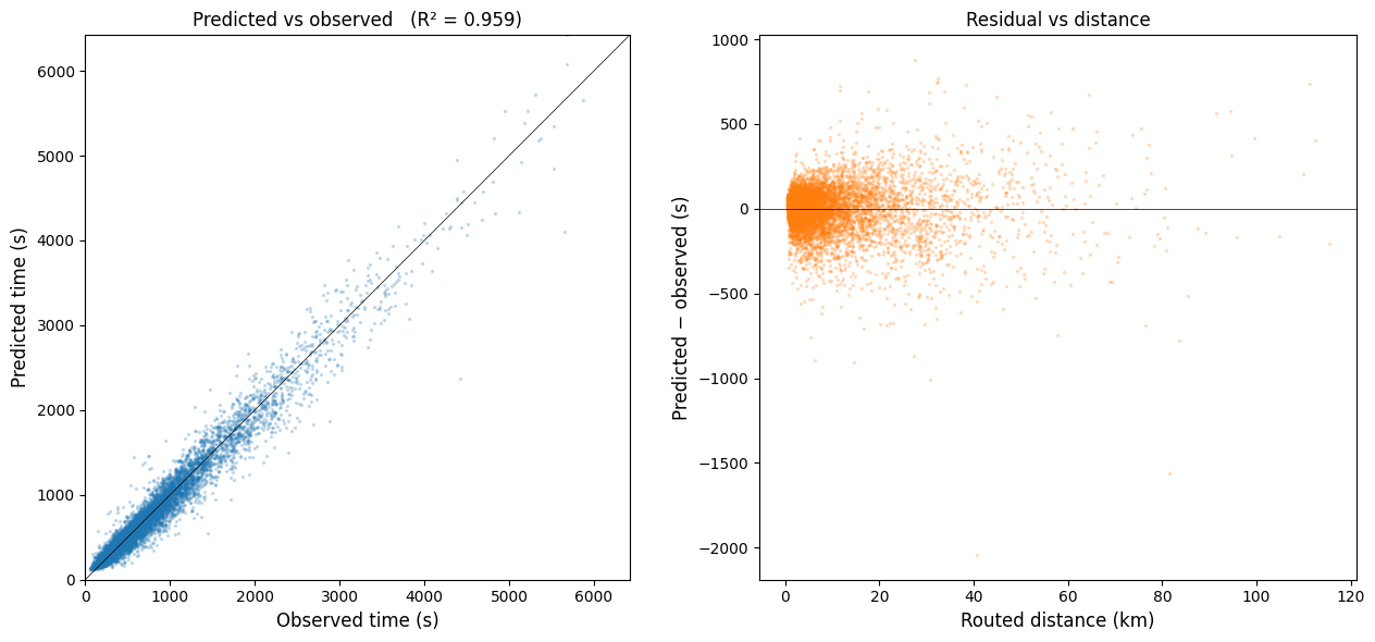
R² = 0.9593   RMSE = 143.7 s   n = 7,460 trips

RMSE by distance band:
< 10 km     112.6
10-25 km    193.9
>= 25 km    296.3

Coefficient table:
                                 kind     coef       p  mean_effect
const                           const  77.5278  0.0000      77.5278
baseline_time                baseline   1.1119  0.0000     676.2699
density_norm__mult         multiplier   0.2966  0.0000      70.1528
is_4way                additive_route   3.6676  0.0000      23.1616
is_traffic_signal      additive_route   6.4283  0.0014       2.8246
snap_dist_orig      additive_endpoint  -0.0111  0.7327      -0.8292
snap_dist_dest      additive_endpoint  -0.0158  0.6256      -1.1842

Iteration log:
           r_squared      rmse  n_used   alpha
iteration
1             0.9593  143.6759    7460  1.1098
2             0.9594  143.4566    7460  0.9987
3             0.9593  143.7305    7460  1.1119

5. Observed vs predicted

import _figures as figures   # noqa: E402
fig, axes = plt.subplots(1, 2, figsize=(13, 6))

# Scatter
ax = axes[0]
ax.scatter(result.observed_times, result.predicted_times,
           s=2, alpha=0.2, color='tab:blue')
lim = max(result.observed_times.max(), result.predicted_times.max())
ax.plot([0, lim], [0, lim], color='black', linewidth=0.5)
ax.set_xlabel('Observed time (s)')
ax.set_ylabel('Predicted time (s)')
ax.set_title(f'Predicted vs observed   (R² = {result.r_squared:.3f})')
ax.set_xlim(0, lim); ax.set_ylim(0, lim)
ax.set_aspect('equal')

# Residual vs distance
ax = axes[1]
residuals = result.predicted_times - result.observed_times
ax.scatter(result.routed_distances / 1000, residuals,
           s=2, alpha=0.2, color='tab:orange')
ax.axhline(0, color='black', linewidth=0.5)
ax.set_xlabel('Routed distance (km)')
ax.set_ylabel('Predicted − observed (s)')
ax.set_title('Residual vs distance')

plt.tight_layout()
figures.save_figure(fig, 'calibration_scatter', ext='pdf')
plt.show()

Saved results/figures_highres/calibration_scatter.pdf

6. Export the calibrated graph

calibrate_edge_weights writes the fitted per-edge duration to car_graph[u][v][k][result.edge_duration_attr] (default 'duration_calibrated') on every edge. The graph is now self-contained — anything that can read GraphML can pick up the calibrated weights.

ox.save_graphml(car_graph, PREPARED_DIR / 'car_graph_calibrated.graphml')

# Companion GeoPackage of edges — opens directly in QGIS / ArcGIS for
# inspection, and serves as a portable cross-tool exchange format.
edges_gdf = ox.graph_to_gdfs(car_graph, nodes=False)
edges_gdf[['length', 'speed_kph', result.edge_duration_attr, 'geometry']].to_file(
    PREPARED_DIR / 'car_edges_calibrated.gpkg', driver='GPKG',
)
print(f"Wrote calibrated graph + edge layer to {PREPARED_DIR}/.")

Wrote calibrated graph + edge layer to data/prepared/.

7. Visualise — per-edge effective speed (calibrated)

Duration is what the calibration fit and what downstream routing consumes, but speed (km/h) is the more intuitive visual: it spreads roads across a familiar 5–120 km/h scale and the colours read as “fast highway” vs “slow congested intersection”. For each edge:

speed_kph = length_m / duration_calibrated_s × 3.6

So intersections and signalised crossings (where calibration added additive seconds) appear as locally slower edges even on a road that OSM tags as a fast through-route — exactly the effect that makes duration_calibrated more realistic than the OSM-maxspeed baseline.

The same numbers live on car_graph_calibrated.graphml (see §6) — downstream consumers can read them per edge from the file directly. Inline computation here so the formula is visible.

# Project-local figure helpers (network map + standardised paper-figure
# crop). Same centre + 20×20 km extent as the other paper figures.
import _figures as figures   # noqa: E402

PAPER_CROP_CENTER_XY = (2_599_000, 1_200_500)
PAPER_CROP_HALF_M    = 15_000

speed_calibrated_kph = {
    (u, v, k): float(d['length']) / float(d[result.edge_duration_attr]) * 3.6
    for u, v, k, d in car_graph.edges(keys=True, data=True)
    if float(d[result.edge_duration_attr]) > 0
}
_speeds = np.array(list(speed_calibrated_kph.values()))
print(f"Calibrated edge speeds (km/h): "
      f"median {np.median(_speeds):.1f}, "
      f"P5–P95 [{np.quantile(_speeds, 0.05):.1f}, "
      f"{np.quantile(_speeds, 0.95):.1f}], "
      f"max {_speeds.max():.0f}")

fig, ax = plt.subplots(figsize=(7, 6.5))
figures.plot_network_map(
    ax, car_graph, speed_calibrated_kph,
    cmap='YlGnBu',                  # low = slow, high = fast
    vmin=10, vmax=90,
    cbar_label='effective speed (km/h, including intersections)',
    title='Calibrated per-edge average effective speed (peak hours)',
    xlim=(PAPER_CROP_CENTER_XY[0] - PAPER_CROP_HALF_M,
          PAPER_CROP_CENTER_XY[0] + PAPER_CROP_HALF_M),
    ylim=(PAPER_CROP_CENTER_XY[1] - PAPER_CROP_HALF_M,
          PAPER_CROP_CENTER_XY[1] + PAPER_CROP_HALF_M),
    basemap=True, crs=CRS_METRIC,
)
plt.tight_layout()
figures.save_figure(fig, 'calibrated_edge_speed_map')
plt.show()

Calibrated edge speeds (km/h): median 26.1, P5–P95 [19.5, 55.6], max 106
Saved results/figures_highres/calibrated_edge_speed_map.png

Consuming the calibrated weights from Pandana

Pandana is a fast C++ routing engine widely used for cumulative-opportunity accessibility. Aperta and Pandana are complementary: aperta produces calibrated, multi-modal, behaviour-anchored edge weights; Pandana consumes them for high-throughput single-mode shortest-path queries on a fixed network.

import osmnx as ox
import pandana
import pandas as pd

g = ox.load_graphml('data/prepared/car_graph_calibrated.graphml')
nodes = ox.graph_to_gdfs(g, edges=False)
edges = ox.graph_to_gdfs(g, nodes=False).reset_index()

net = pandana.Network(
    node_x=nodes['x'], node_y=nodes['y'],
    edge_from=edges['u'], edge_to=edges['v'],
    edge_weights=edges[['duration_calibrated']],
)
net.set(pd.Series(supermarket_node_ids, index=supermarket_node_ids),
        name='supermarkets')
n_within_15min = net.aggregate(
    distance=15 * 60, type='count', name='supermarkets',
)

The same .graphml loads into NetworkX, igraph, r5py, and any custom Dijkstra implementation. Calibration is a one-time step whose product is a standard graph file — downstream tooling is the caller’s choice.

What this notebook does NOT do

This is a self-contained demo of one library capability — calibrating per-edge durations against observed point-to-point travel times. To keep it readable as a tutorial, it deliberately omits things that matter for production:

• No flows / traffic-flow features. The library’s calibrate_edge_weights accepts arbitrary multiplier features, so a flow_estimate AADT estimate (see traffic_flows.ipynb) can enter through a BPR-style (V/C)² transform to capture congestion. The production lumos pipeline does this. Showcase keeps the model interpretable.

• No iterative refinement on stricter trip filters. Production typically iterates filters (drop trip outliers, retain only trips within a polygon, etc.) — we use a single set here.

• Export not consumed by ``accessibility.ipynb``. The calibrated GraphML written in §6 isn’t picked up by the other notebooks — accessibility.ipynb uses published-paper coefficients instead. Each showcase notebook stands alone; they aren’t wired into a pipeline.

For an example of these pieces wired into a full production stack with aperta_lab scaffolding (scenario configs, typed I/O, dependency tracking), see `aperta-lab/src/projects/lumos/calibration/ <https://github.com/mmiotti/aperta-lab/tree/main/src/projects/lumos/calibration>`__.